In this article we illustrate how to fit cause specific hazards models to competing risks data. The standard way to estimate cause specific hazards is to create one data set for each event type and fit a separate model. However, it is also possible to create one combined data set and enter the event type as a covariate (with interactions), such that it is possible to estimate shared effects (i.e., effects that contribute equally to the hazard of multiple event types).
For illustration we use the fourD data set from the etm package. The data set contains time-constant covariates like age and sex as well as time-to-event (time) and event type indicator status (0 = censored, 1 = death from cardiovascular events, 2 = death from other causes).
##      id    sex age medication status      time treated
## 1  5002   Male  60    Placebo      0 5.8480493       0
## 4  5006 Female  68    Placebo      0 5.2539357       0
## 7  5011 Female  70    Placebo      1 2.9541410       0
## 9  5014   Male  69    Placebo      1 0.9856263       0
## 10 5017 Female  58    Placebo      1 0.2902122       0
## 11 5018   Male  63    Placebo      1 3.9452430       0
Cause specific hazards model without shared effects
Below we transform the data set for the case without shared effects. By specifying cobmine = FALSE, the individual data sets are not stacked but rather returned in a list.
cut <- sample(fourD$time, 100)
ped <- fourD %>%
  select(-medication, - treated) %>%
  as_ped(Surv(time, status)~., id = "id", cut = cut, combine = FALSE)
str(ped, 1)
## List of 2
##  $ cause = 1:Classes 'ped' and 'data.frame': 31367 obs. of  9 variables:
##   ..- attr(*, "breaks")= num [1:100] 0.052 0.194 0.208 0.274 0.312 ...
##   ..- attr(*, "id_var")= chr "id"
##   ..- attr(*, "intvars")= chr [1:6] "id" "tstart" "tend" "interval" ...
##   ..- attr(*, "trafo_args")=List of 3
##   ..- attr(*, "time_var")= chr "time"
##   ..- attr(*, "status_var")= chr "status"
##  $ cause = 2:Classes 'ped' and 'data.frame': 31367 obs. of  9 variables:
##   ..- attr(*, "breaks")= num [1:100] 0.052 0.194 0.208 0.274 0.312 ...
##   ..- attr(*, "id_var")= chr "id"
##   ..- attr(*, "intvars")= chr [1:6] "id" "tstart" "tend" "interval" ...
##   ..- attr(*, "trafo_args")=List of 3
##   ..- attr(*, "time_var")= chr "time"
##   ..- attr(*, "status_var")= chr "status"
##  - attr(*, "class")= chr [1:4] "ped_cr_list" "ped_cr" "ped" "list"
##  - attr(*, "trafo_args")=List of 5
##  - attr(*, "risks")= int [1:2] 1 2
# data set for event type 1 (death from cardiovascular events)
head(ped[[1]])
##     id     tstart       tend                    interval    offset ped_status
## 1 5002 0.00000000 0.05201916             (0,0.052019165] -2.956143          0
## 2 5002 0.05201916 0.19438741  (0.052019165,0.1943874059] -1.949338          0
## 3 5002 0.19438741 0.20807666 (0.1943874059,0.2080766598] -4.291144          0
## 4 5002 0.20807666 0.27378508 (0.2080766598,0.2737850787] -2.722528          0
## 5 5002 0.27378508 0.31211499 (0.2737850787,0.3121149897] -3.261525          0
## 6 5002 0.31211499 0.39698836 (0.3121149897,0.3969883641] -2.466595          0
##    sex age cause
## 1 Male  60     1
## 2 Male  60     1
## 3 Male  60     1
## 4 Male  60     1
## 5 Male  60     1
## 6 Male  60     1
# data set for event type 2 (death from other causes)
head(ped[[2]])
##     id     tstart       tend                    interval    offset ped_status
## 1 5002 0.00000000 0.05201916             (0,0.052019165] -2.956143          0
## 2 5002 0.05201916 0.19438741  (0.052019165,0.1943874059] -1.949338          0
## 3 5002 0.19438741 0.20807666 (0.1943874059,0.2080766598] -4.291144          0
## 4 5002 0.20807666 0.27378508 (0.2080766598,0.2737850787] -2.722528          0
## 5 5002 0.27378508 0.31211499 (0.2737850787,0.3121149897] -3.261525          0
## 6 5002 0.31211499 0.39698836 (0.3121149897,0.3969883641] -2.466595          0
##    sex age cause
## 1 Male  60     2
## 2 Male  60     2
## 3 Male  60     2
## 4 Male  60     2
## 5 Male  60     2
## 6 Male  60     2
To fit the model, we could loop through the list entries and fit the model of interest, however, there is also a convenience function, that recognizes the data type and fits the models accordingly:
library(mgcv)
pam_csh <- map(ped, ~ pamm(ped_status ~ s(tend) + sex + age, data = .x))
map(pam_csh, summary)
## $`cause = 1`
##
## Family: poisson
## Link function: log
##
## Formula:
## ped_status ~ s(tend) + sex + age
##
## Parametric coefficients:
##              Estimate Std. Error z value Pr(>|z|)
## (Intercept) -3.222913   0.581605  -5.541    3e-08 ***
## sexMale     -0.135535   0.131152  -1.033   0.3014
## age          0.021008   0.008416   2.496   0.0126 *
## ---
## Signif. codes:  0 '***' 0.001 '**' 0.01 '*' 0.05 '.' 0.1 ' ' 1
##
## Approximate significance of smooth terms:
##           edf Ref.df Chi.sq p-value
## s(tend) 1.005   1.01  8.457 0.00372 **
## ---
## Signif. codes:  0 '***' 0.001 '**' 0.01 '*' 0.05 '.' 0.1 ' ' 1
##
## R-sq.(adj) =  -0.00971   Deviance explained = 0.59%
## UBRE = -0.91361  Scale est. = 1         n = 31367
##
## $`cause = 2`
##
## Family: poisson
## Link function: log
##
## Formula:
## ped_status ~ s(tend) + sex + age
##
## Parametric coefficients:
##             Estimate Std. Error z value Pr(>|z|)
## (Intercept) -6.95859    0.88235  -7.886 3.11e-15 ***
## sexMale      0.16758    0.18028   0.930    0.353
## age          0.06426    0.01244   5.165 2.40e-07 ***
## ---
## Signif. codes:  0 '***' 0.001 '**' 0.01 '*' 0.05 '.' 0.1 ' ' 1
##
## Approximate significance of smooth terms:
##           edf Ref.df Chi.sq p-value
## s(tend) 1.013  1.026  10.73 0.00111 **
## ---
## Signif. codes:  0 '***' 0.001 '**' 0.01 '*' 0.05 '.' 0.1 ' ' 1
##
## R-sq.(adj) =  -0.00243   Deviance explained = 2.39%
## UBRE = -0.95265  Scale est. = 1         n = 31367
Cause specific hazards with shared effects
The data transformation is performed as before, but setting combine=TRUE (the default), the interval cut points are created based on all event times (event times of all event types, here) and stacked:
##     id     tstart       tend                    interval    offset ped_status
## 1 5002 0.00000000 0.05201916             (0,0.052019165] -2.956143          0
## 2 5002 0.05201916 0.19438741  (0.052019165,0.1943874059] -1.949338          0
## 3 5002 0.19438741 0.20807666 (0.1943874059,0.2080766598] -4.291144          0
## 4 5002 0.20807666 0.27378508 (0.2080766598,0.2737850787] -2.722528          0
## 5 5002 0.27378508 0.31211499 (0.2737850787,0.3121149897] -3.261525          0
## 6 5002 0.31211499 0.39698836 (0.3121149897,0.3969883641] -2.466595          0
##    sex age cause
## 1 Male  60     1
## 2 Male  60     1
## 3 Male  60     1
## 4 Male  60     1
## 5 Male  60     1
## 6 Male  60     1
Model for cause specific hazards with shared effects is performed by inclusion of interaction effects:
pam_csh_shared <- pamm(
  formula = ped_status ~ s(tend, by = cause) + sex + sex:cause + age + age:cause,
  data = ped_stacked)
summary(pam_csh_shared)
##
## Family: poisson
## Link function: log
##
## Formula:
## ped_status ~ s(tend, by = cause) + sex + sex:cause + age + age:cause
##
## Parametric coefficients:
##                   Estimate Std. Error z value Pr(>|z|)
## (Intercept)      -3.144778   0.583239  -5.392 6.97e-08 ***
## sexMale          -0.131260   0.132001  -0.994 0.320033
## age               0.019735   0.008445   2.337 0.019442 *
## sexFemale:cause2 -3.808175   1.057883  -3.600 0.000318 ***
## sexMale:cause2   -3.509432   1.011478  -3.470 0.000521 ***
## age:cause2        0.044544   0.015038   2.962 0.003055 **
## ---
## Signif. codes:  0 '***' 0.001 '**' 0.01 '*' 0.05 '.' 0.1 ' ' 1
##
## Approximate significance of smooth terms:
##                  edf Ref.df Chi.sq p-value
## s(tend):cause1 1.006  1.011  7.746 0.00550 **
## s(tend):cause2 1.042  1.082 10.569 0.00134 **
## ---
## Signif. codes:  0 '***' 0.001 '**' 0.01 '*' 0.05 '.' 0.1 ' ' 1
##
## R-sq.(adj) =  -0.00666   Deviance explained = 2.04%
## UBRE = -0.93185  Scale est. = 1         n = 60910
The results indicate that cause specific terms (interactions) are necessary in this case and the two models largely agree. For example, the age effect for the two causes are very similar for both models:
- cause1: 0.021 (
pamm_csh1) vs. 0.02 (pamm_csh_shared)
- cause2: 0.064 (
pamm_csh2) vs. 0.02 + 0.045= 0.065 (pamm_csh_shared)
Cumulative Incidence Function (CIF)
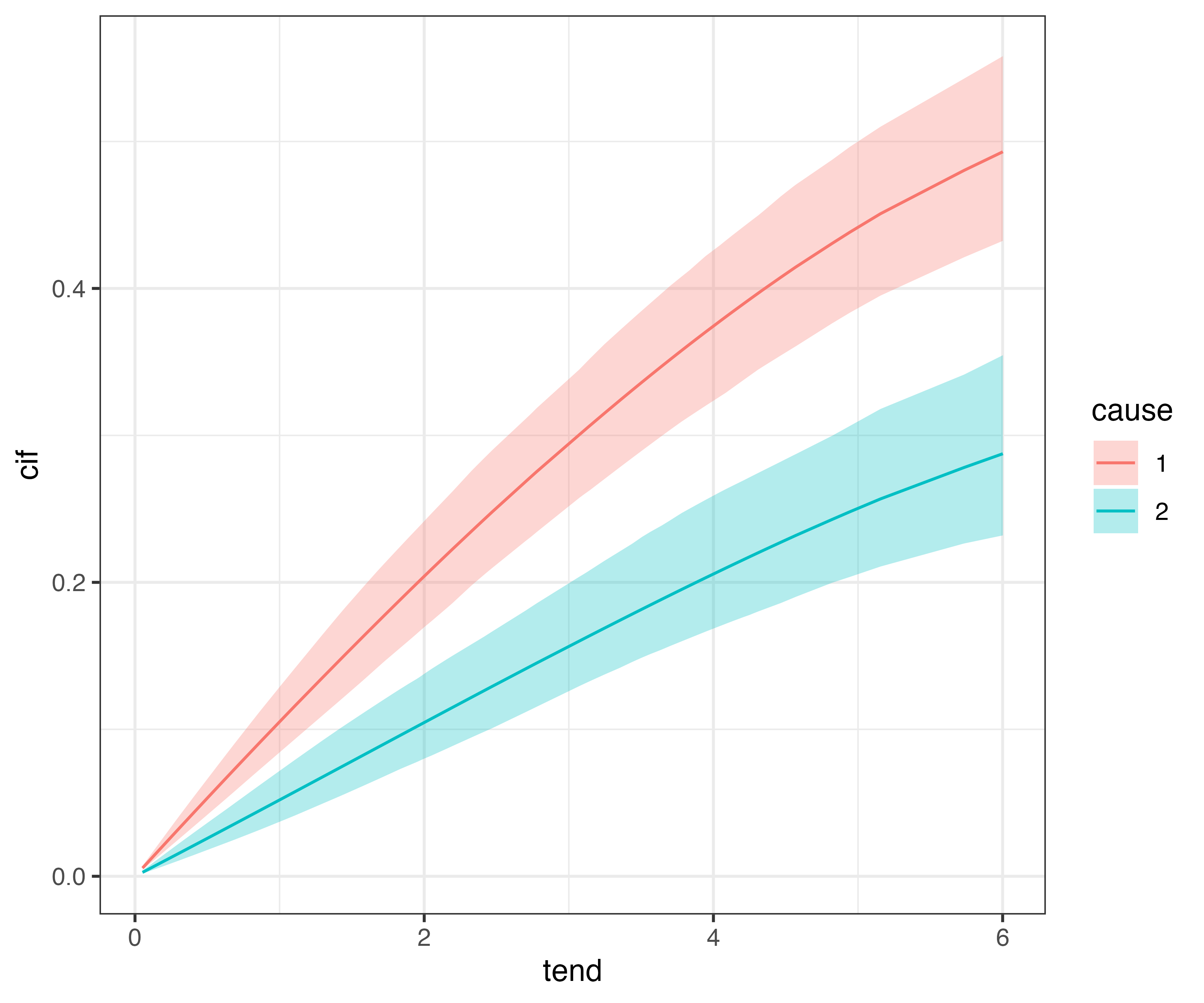
Finally, in many cases we will want to calculate and visualize the cumulative incidence functions for different covariate combinations. In pammtools this can be again achieved using make_newdata and using the appropriate add_* function, here add_cif:
## # A tibble: 6 x 5
## # Groups:   cause [2]
##     tend cause     cif cif_lower cif_upper
##    <dbl> <fct>   <dbl>     <dbl>     <dbl>
## 1 0.0520 1     0.00559   0.00433   0.00710
## 2 0.194  1     0.0208    0.0162    0.0262
## 3 0.208  1     0.0223    0.0173    0.0280
## 4 0.0520 2     0.00267   0.00178   0.00388
## 5 0.194  2     0.00999   0.00679   0.0143
## 6 0.208  2     0.0107    0.00728   0.0153
Similar to other applications of add_* functions, we can additionally group by other covariate values:
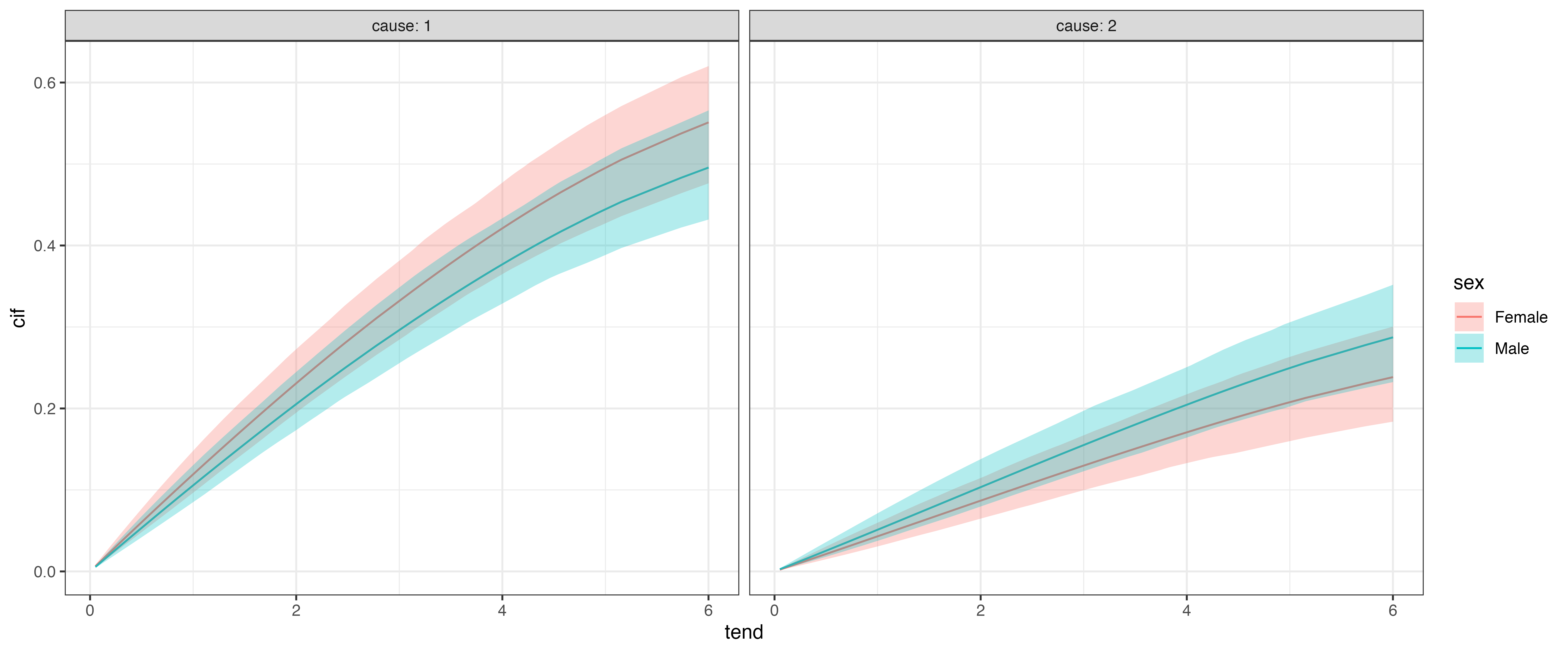
The estimated CIFs can then be compared w.r.t. to cause for each category of sex:
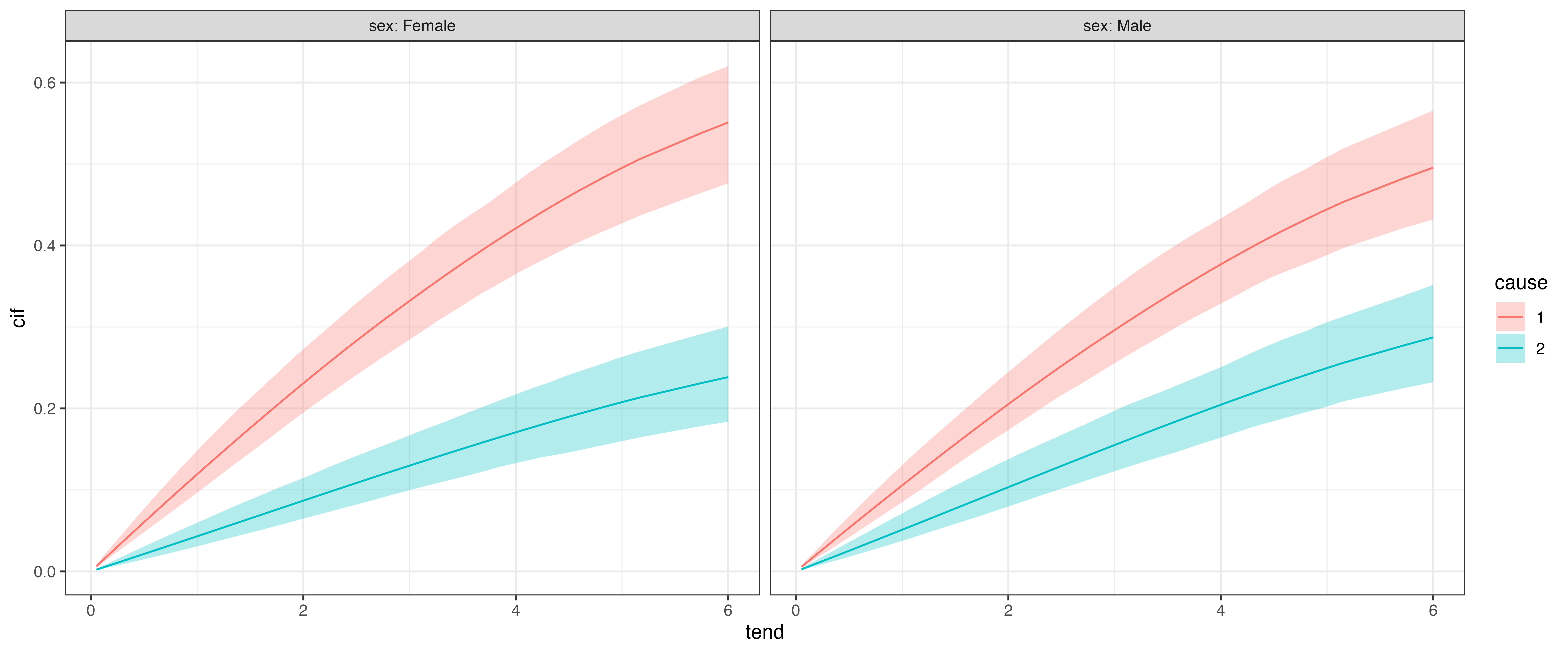
or w.r.t. to sex for each cause: