Simulate survival times from the piece-wise exponential distribution

sim_pexp(formula, data, cut)

Arguments

formula	An extended formula that specifies the linear predictor. If you want to include a smooth baseline or time-varying effects, use `t` within your formula as if it was a covariate in the data, although it is not and should not be included in the `data` provided to `sim_pexp`. See examples below.
data	A data set with variables specified in `formula`.
cut	A sequence of time-points starting with 0.

Examples

library(survival)
library(dplyr)
#> 
#> Attaching package: ‘dplyr’
#> The following objects are masked from ‘package:stats’:
#> 
#>     filter, lag
#> The following objects are masked from ‘package:base’:
#> 
#>     intersect, setdiff, setequal, union
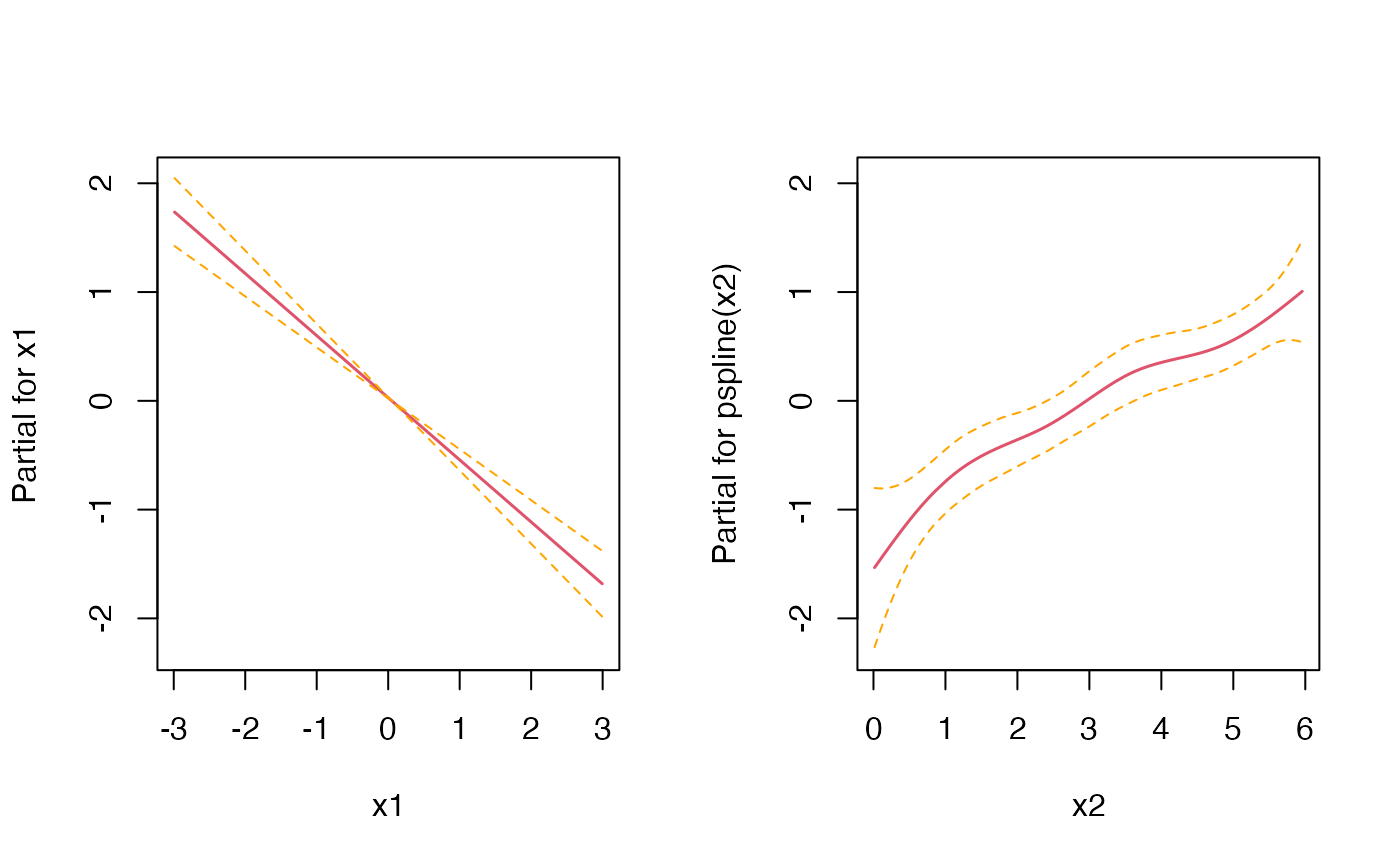
library(pammtools)

# set number of observations/subjects
n <- 250
# create data set with variables which will affect the hazard rate.
df <- cbind.data.frame(x1 = runif (n, -3, 3), x2 = runif (n, 0, 6)) %>%
 as_tibble()
# the formula which specifies how covariates affet the hazard rate
f0 <- function(t) {
 dgamma(t, 8, 2) *6
}
form <- ~ -3.5 + f0(t) -0.5*x1 + sqrt(x2)
set.seed(24032018)
sim_df <- sim_pexp(form, df, 1:10)
head(sim_df)
#> # A tibble: 6 x 5
#>      id  time status     x1    x2
#>   <int> <dbl>  <int>  <dbl> <dbl>
#> 1     1  1.00      1 -2.87   4.14
#> 2     2  4.20      1  1.20   5.61
#> 3     3  4.53      1 -0.951  2.46
#> 4     4  2.07      1  0.331  3.71
#> 5     5  3.02      1  2.98   4.98
#> 6     6  2.32      1 -1.91   1.43
plot(survfit(Surv(time, status)~1, data = sim_df ))

# for control, estimate with Cox PH
mod <- coxph(Surv(time, status) ~ x1 + pspline(x2), data=sim_df)
coef(mod)[1]
#>         x1 
#> -0.5711059 
layout(matrix(1:2, nrow=1))
termplot(mod, se = TRUE)

# and using PAMs
layout(1)
ped <- sim_df %>% as_ped(Surv(time, status)~., max_time=10)
library(mgcv)
#> Loading required package: nlme
#> 
#> Attaching package: ‘nlme’
#> The following object is masked from ‘package:dplyr’:
#> 
#>     collapse
#> This is mgcv 1.8-35. For overview type 'help("mgcv-package")'.
pam <- gam(ped_status ~ s(tend) + x1 + s(x2), data=ped, family=poisson, offset=offset)
coef(pam)[2]
#>         x1 
#> -0.5534093 
plot(pam, page=1)

if (FALSE) {
# Example 2: Functional covariates/cumulative coefficients
# function to generate one exposure profile, tz is a vector of time points
# at which TDC z was observed
rng_z = function(nz) {
  as.numeric(arima.sim(n = nz, list(ar = c(.8, -.6))))
}
# two different exposure times  for two different exposures
tz1 <- 1:10
tz2 <- -5:5
# generate exposures and add to data set
df <- df %>%
  add_tdc(tz1, rng_z) %>%
  add_tdc(tz2, rng_z)
df

# define tri-variate function of time, exposure time and exposure z
ft <- function(t, tmax) {
  -1*cos(t/tmax*pi)
}
fdnorm <- function(x) (dnorm(x,1.5,2)+1.5*dnorm(x,7.5,1))
wpeak2 <- function(lag) 15*dnorm(lag,8,10)
wdnorm <- function(lag) 5*(dnorm(lag,4,6)+dnorm(lag,25,4))
f_xyz1 <- function(t, tz, z) {
  ft(t, tmax=10) * 0.8*fdnorm(z)* wpeak2(t - tz)
}
f_xyz2 <- function(t, tz, z) {
  wdnorm(t-tz) * z
}

# define lag-lead window function
ll_fun <- function(t, tz) {t >= tz}
ll_fun2 <- function(t, tz) {t - 2 >= tz}
# simulate data with cumulative effect
sim_df <- sim_pexp(
  formula = ~ -3.5 + f0(t) -0.5*x1 + sqrt(x2)|
     fcumu(t, tz1, z.tz1, f_xyz=f_xyz1, ll_fun=ll_fun) +
     fcumu(t, tz2, z.tz2, f_xyz=f_xyz2, ll_fun=ll_fun2),
  data = df,
  cut = 0:10)
}