LOCO and LOCI • xplainfi

library(xplainfi)
library(mlr3)
library(mlr3learners)
library(data.table)
library(ggplot2)

Example Data: Interaction Effects

To illustrate the key differences between LOCO and LOCI, we’ll use a data generating process with interaction effects:

\[y = 2 \cdot x_1 \cdot x_2 + x_3 + \epsilon\]

where $\epsilon \sim N(0, 0.5^2)$ and all features $x_1, x_2, x_3, noise_1, noise_2 \sim N(0,1)$ are independent.

Key characteristics:

$x_1, x_2$: Have NO individual effects, only interact with each other
$x_3$: Has a direct main effect on $y$
$noise_1, noise_2$: Pure noise variables with no effect on $y$

This setup highlights how LOCO and LOCI handle interaction effects differently.

Leave-One-Covariate-Out (LOCO)

LOCO measures feature importance by comparing model performance with and without each feature. For each feature, the learner is retrained without that feature and the performance difference indicates the feature’s importance.

For feature $j$, LOCO is calculated as the difference in expected loss of the model fit without the feature and the full model: \[\text{LOCO}_j = \mathbb{E}(L(Y, f_{-j}(X_{-j}))) - \mathbb{E}(L(Y, f(X)))\]

Higher values indicate more important features (larger performance drop when removed).

task <- sim_dgp_interactions(n = 500)
learner <- lrn("regr.lm")
measure <- msr("regr.mse")

loco <- LOCO$new(
  task = task,
  learner = learner,
  measure = measure
)
#> ℹ No <Resampling> provided
#> Using `resampling = rsmp("holdout")` with default `ratio = 0.67`.

loco$compute()
loco$importance()
#> Key: <feature>
#>    feature  importance
#>     <char>       <num>
#> 1:  noise1  0.02343712
#> 2:  noise2  0.01808013
#> 3:      x1 -0.14135998
#> 4:      x2  0.11463314
#> 5:      x3  0.65082799

Leave-One-Covariate-In (LOCI)

LOCI measures feature importance by training models with only each individual feature and comparing their performance to a featureless (baseline) model. This shows how much predictive power each feature provides on its own, above and beyond the optimal constant prediction.

Since this method only measures univariate associations, it is not recommend to use as a “real” feature importance method, but rather exists as a special case of a broader class of refitting-based importances methods. We illustrate it here for completeness and to highlight its limitation.

For feature $j$, LOCI is calculated as the difference in expected loss of the featureless learner or constant model and the model including only the feature: \[\text{LOCI}_j = \mathbb{E}(L(Y, f_{\emptyset})) - \mathbb{E}(L(Y, f_j(X_{j})))\]

Higher values indicate more important features (better individual performance compared to baseline).

loci <- LOCI$new(
  task = task,
  learner = learner,
  measure = measure
)
#> ℹ No <Resampling> provided
#> Using `resampling = rsmp("holdout")` with default `ratio = 0.67`.

loci$compute()
loci$importance()
#> Key: <feature>
#>    feature  importance
#>     <char>       <num>
#> 1:  noise1  0.09848467
#> 2:  noise2 -0.05579254
#> 3:      x1 -0.44010340
#> 4:      x2  0.11155710
#> 5:      x3  0.58359019

Understanding the Results

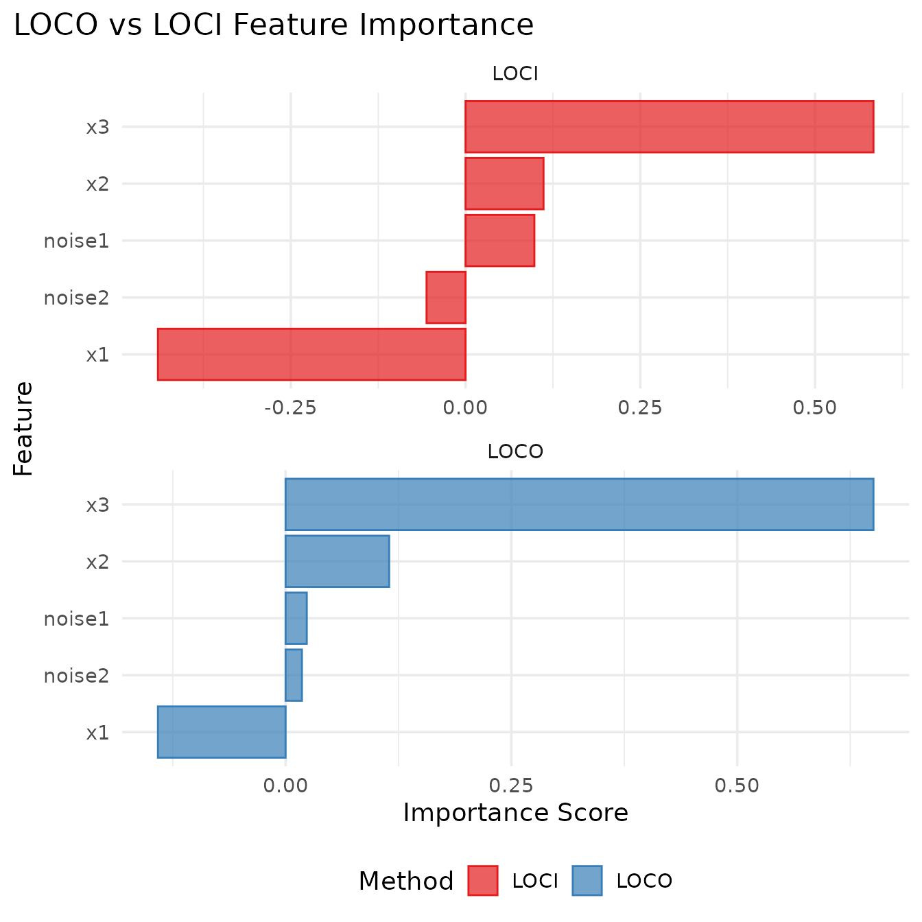
LOCO results interpretation:

$x_1$ and $x_2$ show low importance because removing either one eliminates the interaction ($x_1 \cdot x_2$ becomes zero)
$x_3$ shows higher importance due to its direct main effect
This demonstrates LOCO’s limitation with interaction effects

LOCI results interpretation:

$x_1$ and $x_2$ show low importance because individually they have no predictive power
$x_3$ shows high importance because it alone can predict $y$ reasonably well
This shows how LOCI focuses on individual feature contributions

Multiple Refits

Like PFI has iters_perm for multiple permutation iterations, LOCO and LOCI support iters_refit for multiple refit iterations per resampling iteration, which then also provide standard deviations:

loco_multi = LOCO$new(
  task = task,
  learner = learner,
  measure = measure,
  resampling = rsmp("cv", folds = 3),
  iters_refit = 3L
)

loco_multi$compute()
loco_multi$importance()
#> Key: <feature>
#>    feature  importance
#>     <char>       <num>
#> 1:  noise1 -0.01212711
#> 2:  noise2 -0.02467126
#> 3:      x1 -0.08943524
#> 4:      x2 -0.07556117
#> 5:      x3  0.82401461

# Check individual scores with multiple refits
loco_multi$scores[1:10, ] |>
  knitr::kable(digits = 4, caption = "LOCO scores per refit and resampling fold")

LOCO scores per refit and resampling fold
feature	iter_rsmp	iter_refit	regr.mse_orig	regr.mse_post	importance
noise1	1	1	3.8491	3.7693	-0.0798
noise1	1	2	3.8491	3.7693	-0.0798
noise1	1	3	3.8491	3.7693	-0.0798
noise1	2	1	4.2981	4.3134	0.0153
noise1	2	2	4.2981	4.3134	0.0153
noise1	2	3	4.2981	4.3134	0.0153
noise1	3	1	5.3040	5.3321	0.0281
noise1	3	2	5.3040	5.3321	0.0281
noise1	3	3	5.3040	5.3321	0.0281
noise2	1	1	3.8491	3.7563	-0.0928

Comparing LOCO and LOCI

# Combine results for comparison
importance_combined <- rbind(
  loco$importance()[, method := "LOCO"],
  loci$importance()[, method := "LOCI"]
)

importance_combined <- importance_combined |>
  dcast(feature ~ method, value.var = "importance")

importance_combined |>
  knitr::kable(digits = 4, caption = "LOCO vs LOCI importance scores")

LOCO vs LOCI importance scores
feature	LOCI	LOCO
noise1	0.0985	0.0234
noise2	-0.0558	0.0181
x1	-0.4401	-0.1414
x2	0.1116	0.1146
x3	0.5836	0.6508

Interpreting the results:

LOCO: Higher values indicate more important features (larger performance drop when removed)
LOCI: Higher values indicate more important features (better individual performance compared to baseline)
- Positive values: feature performs better than featureless baseline
- Negative values: feature performs worse than featureless baseline

Different aggregation methods in LOCO

The examples above aggregates predictions on each test set (obs_loss = FALSE), computing importance as the difference of average losses using the measure’s default aggregation: $\mathrm{mean}(L(Y, f_{-j}(X_{-j}))) - \mathrm{mean}(L(Y, f(X)))$.

LOCO can also be computed using the alternative approach (obs_loss = TRUE), which follows the original paper formulation by aggregating observation-wise differences. The aggregation function is taken from the measure’s aggregator field (defaulting to mean if not specified). For the original LOCO formulation with median of absolute differences, we can customize the measure’s aggregator: $\mathrm{median}(\{|L(y_i, f_{-j}(x_{i,-j}))| - |L(y_i, f(x_i))|\}_{i=1}^n)$, where we use an mlr3 measure with $L_1$ loss on the observation level, e.g regr.mae.

Setting obs_loss = TRUE provides access to individual observation-level differences:

# Use macro-averaged approach with median aggregation
# Create MAE measure with median aggregator for original LOCO formulation
mae_median <- msr("regr.mae")
mae_median$aggregator <- median

loco_obs <- LOCO$new(
  task = task,
  learner = learner,
  measure = mae_median,  # MAE with median aggregator
  obs_loss = TRUE
)
#> ℹ No <Resampling> provided
#> Using `resampling = rsmp("holdout")` with default `ratio = 0.67`.

loco_obs$compute()
loco_obs$importance()
#> Key: <feature>
#>    feature   importance
#>     <char>        <num>
#> 1:  noise1  0.001274411
#> 2:  noise2  0.003229655
#> 3:      x1  0.001995886
#> 4:      x2 -0.077958164
#> 5:      x3  0.315709247

# Compare aggregated results
rbind(
  loco$importance()[, method := "Set-wise MSE (measure default)"],
  loco_obs$importance()[, method := "Observation-wise (median of diffs)"]
) |>
  dcast(feature ~ method, value.var = "importance") |>
  knitr::kable(digits = 4, caption = "Comparison of LOCO aggregation approaches")

Comparison of LOCO aggregation approaches
feature	Observation-wise (median of diffs)	Set-wise MSE (measure default)
noise1	0.0013	0.0234
noise2	0.0032	0.0181
x1	0.0020	-0.1414
x2	-0.0780	0.1146
x3	0.3157	0.6508

The $obs_losses field provides detailed observation-level information:

# Examine observation-wise data for first feature
feature_data <- loco_obs$obs_losses[feature == "x3"]

# Show structure
str(feature_data)
#> Classes 'data.table' and 'data.frame':   167 obs. of  10 variables:
#>  $ row_ids         : int  3 4 5 6 8 9 11 12 13 15 ...
#>  $ feature         : chr  "x3" "x3" "x3" "x3" ...
#>  $ iteration       : int  1 1 1 1 1 1 1 1 1 1 ...
#>  $ iter_refit      : int  1 1 1 1 1 1 1 1 1 1 ...
#>  $ truth           : num  2.831 -0.293 -2.552 0.476 8.165 ...
#>  $ response_ref    : num  0.468 0.0826 -2.7257 0.7273 1.0292 ...
#>  $ response_feature: num  0.828 0.247 -0.983 -0.334 -0.975 ...
#>  $ loss_ref        : num  2.363 0.376 0.173 0.251 7.136 ...
#>  $ loss_feature    : num  2.003 0.541 1.569 0.81 9.14 ...
#>  $ obs_diff        : num  -0.36 0.165 1.396 0.559 2.004 ...
#>  - attr(*, ".internal.selfref")=<externalptr>

# Display first few observations
head(feature_data) |>
  knitr::kable(digits = 3, caption = "Observation-wise losses for x3")

Observation-wise losses for x3
row_ids	feature	iteration	iter_refit	truth	response_ref	response_feature	loss_ref	loss_feature	obs_diff
3	x3	1	1	2.831	0.468	0.828	2.363	2.003	-0.360
4	x3	1	1	-0.293	0.083	0.247	0.376	0.541	0.165
5	x3	1	1	-2.552	-2.726	-0.983	0.173	1.569	1.396
6	x3	1	1	0.476	0.727	-0.334	0.251	0.810	0.559
8	x3	1	1	8.165	1.029	-0.975	7.136	9.140	2.004
9	x3	1	1	-0.124	0.415	-0.205	0.539	0.081	-0.458

Each row contains:

row_ids: Test set observation identifiers
truth: Original target values
response_ref: Full model predictions
response_feature: Reduced model predictions (without this feature)
loss_ref / loss_feature: Individual losses from each model
obs_diff: Observation-wise importance differences

Note that when using regr.mse (which aggregates with the mean) for observation-wise losses, both approaches yield the same result, but in slightly different ways:

set.seed(1)
resampling = rsmp("holdout")
resampling$instantiate(task)

loco_orig <- LOCO$new(
  task = task,
  learner = learner,
  resampling = resampling,
  measure = measure
)

loco_obsloss <- LOCO$new(
  task = task,
  learner = learner,
  resampling = resampling,
  measure = measure,  # MSE uses mean by default
  obs_loss = TRUE
)

rbind(
  {loco_orig$compute(); loco_orig$importance()[, method := "Set-wise"]},
  {loco_obsloss$compute(); loco_obsloss$importance()[, method := "Observation-wise"]}
) |>
  dcast(feature ~ method, value.var = "importance")
#> Key: <feature>
#>    feature Observation-wise    Set-wise
#>     <char>            <num>       <num>
#> 1:  noise1      -0.06116845 -0.06116845
#> 2:  noise2      -0.03037297 -0.03037297
#> 3:      x1      -0.04521521 -0.04521521
#> 4:      x2       0.02801885  0.02801885
#> 5:      x3       1.10230314  1.10230314

Classification Example with Probability Access

For classification tasks, the obs_losses field stores predicted classes while preserving access to probabilities from the original mlr3 prediction objects:

# Binary classification task
task_classif <- tgen("circle", d = 6)$generate(n = 200)

# Learner with probability predictions (required for accessing probabilities later)
learner_classif <- lrn("classif.rpart", predict_type = "prob")

# LOCO with observation-wise losses
loco_classif <- LOCO$new(
  task = task_classif,
  learner = learner_classif,
  measure = msr("classif.ce"),  # Classification error supports obs_loss (zero-one in this case)
  obs_loss = TRUE,
  features = c("x1", "x2")  # Focus on just two features for clarity
)
#> ℹ No <Resampling> provided
#> Using `resampling = rsmp("holdout")` with default `ratio = 0.67`.

loco_classif$compute()
loco_classif$importance()
#> Key: <feature>
#>    feature importance
#>     <char>      <num>
#> 1:      x1 0.04477612
#> 2:      x2 0.00000000

# Show classification importance
loco_classif$importance() |>
  knitr::kable(digits = 4, caption = "LOCO importance for classification")

LOCO importance for classification
feature	importance
x1	0.0448
x2	0.0000

Examine the observation-wise classification results:

# Look at observation-wise data
classif_data <- head(loco_classif$obs_losses, 8)

classif_data |>
  knitr::kable(caption = "Observation-wise classification losses")

Observation-wise classification losses
row_ids	feature	iteration	iter_refit	truth	response_ref	response_feature
5	x1	1	1	B	B	B
5	x2	1	1	B	B	B
11	x1	1	1	B	B	B
11	x2	1	1	B	B	B
14	x1	1	1	B	B	B
14	x2	1	1	B	B	B
15	x1	1	1	B	B	B
15	x2	1	1	B	B	B

For classification, the response columns contain predicted classes (factors). Note that $resample_result only contains the reference model predictions (full model for LOCO, featureless for LOCI), not the feature-specific models:

# Access feature-specific predictions (available with obs_loss = TRUE)
head(loco_classif$predictions)
#>    feature iteration iter_refit          prediction
#>     <char>     <int>      <int>              <list>
#> 1:      x1         1          1 <PredictionClassif>
#> 2:      x2         1          1 <PredictionClassif>

# Get probabilities for a specific feature and iteration  
if (nrow(loco_classif$predictions) > 0) {
  feature_pred <- loco_classif$predictions[1, ]$prediction[[1]]
  
  # Access both predicted classes and probabilities
  # Note: probabilities are only available because we used predict_type = "prob"
  head(feature_pred$response)  # Predicted classes
  head(feature_pred$prob)      # Probability matrix
}
#>               A         B
#> [1,] 0.06060606 0.9393939
#> [2,] 0.06060606 0.9393939
#> [3,] 0.11111111 0.8888889
#> [4,] 0.09523810 0.9047619
#> [5,] 0.80851064 0.1914894
#> [6,] 0.06060606 0.9393939

# Compare with reference model (full model for LOCO)
ref_pred <- loco_classif$resample_result$prediction(1)
head(ref_pred$prob)  # Reference model probabilities
#>               A          B
#> [1,] 0.06060606 0.93939394
#> [2,] 0.06060606 0.93939394
#> [3,] 0.11111111 0.88888889
#> [4,] 0.09523810 0.90476190
#> [5,] 0.91891892 0.08108108
#> [6,] 0.06060606 0.93939394

The $predictions field provides complete access to feature-specific prediction objects:

feature: Which feature was left out (LOCO) or left in (LOCI)
iteration: Resampling iteration
iter_refit: Refit iteration within resampling
prediction: Complete mlr3 prediction object with responses, probabilities, etc.

This gives you full access to:

Feature-specific probabilities: prediction$prob
Feature-specific predicted classes: prediction$response
Additional prediction data: Any other fields the learner provides

The observation-wise approach is particularly useful for:

Robust aggregation: Using median instead of mean to reduce outlier influence
Individual analysis: Examining which specific observations drive importance scores
Distribution analysis: Understanding the variability in feature effects across observations
Model debugging: Identifying problematic observations or prediction patterns

row_ids	feature	iteration	iter_refit	truth	response_ref	response_feature
5	x1	1	1	B	B	B
5	x2	1	1	B	B	B
11	x1	1	1	B	B	B
11	x2	1	1	B	B	B
14	x1	1	1	B	B	B
14	x2	1	1	B	B	B
15	x1	1	1	B	B	B
15	x2	1	1	B	B	B

row_ids	feature	iteration	iter_refit	truth	response_ref	response_feature
5	x1	1	1	B	B	B
5	x2	1	1	B	B	B
11	x1	1	1	B	B	B
11	x2	1	1	B	B	B
14	x1	1	1	B	B	B
14	x2	1	1	B	B	B
15	x1	1	1	B	B	B
15	x2	1	1	B	B	B

row_ids	feature	iteration	iter_refit	truth	response_ref	response_feature
5	x1	1	1	B	B	B
5	x2	1	1	B	B	B
11	x1	1	1	B	B	B
11	x2	1	1	B	B	B
14	x1	1	1	B	B	B
14	x2	1	1	B	B	B
15	x1	1	1	B	B	B
15	x2	1	1	B	B	B