Shapley Additive Global Importance (SAGE) • xplainfi

library(xplainfi)
library(mlr3)
library(mlr3learners)
library(ggplot2)

Introduction

Shapley Additive Global Importance (SAGE) is a feature importance method based on cooperative game theory that uses Shapley values to fairly distribute the total prediction performance among all features. Unlike permutation-based methods that measure the drop in performance when features are perturbed, SAGE measures how much each feature contributes to the model’s overall performance by marginalizing (removing) features.

The key insight of SAGE is that it provides a complete decomposition of the model’s performance: the sum of all SAGE values equals the difference between the model’s performance and the performance when all features are marginalized.

xplainfi provides two implementations of SAGE:

MarginalSAGE: Marginalizes features independently (standard SAGE)
ConditionalSAGE: Marginalizes features conditionally using ARF sampling

Demonstration with Correlated Features

To showcase the difference between Marginal and Conditional SAGE, we’ll use the sim_dgp_correlated() function which creates highly correlated features. This is similar to how PFI and CFI behave differently with correlated features.

Model: \[X_1 \sim N(0,1)\] \[X_2 = X_1 + \varepsilon_2, \quad \varepsilon_2 \sim N(0, 0.05^2)\] \[X_3 \sim N(0,1), \quad X_4 \sim N(0,1)\] \[Y = 2 \cdot X_1 + X_3 + \varepsilon\]

where \(\varepsilon \sim N(0, 0.2^2)\).

Key properties:

x1 has a direct causal effect on y (β=2.0)
x2 is highly correlated with x1 (r ≈ 0.999) but has no causal effect on y
x3 is independent with a causal effect (β=1.0)
x4 is independent noise (β=0)

set.seed(123)
task = sim_dgp_correlated(n = 800)

# Check the correlation structure
task_data = task$data()
correlation_matrix = cor(task_data[, c("x1", "x2", "x3", "x4")])
round(correlation_matrix, 3)
#>        x1     x2     x3     x4
#> x1  1.000  0.999  0.041 -0.024
#> x2  0.999  1.000  0.039 -0.020
#> x3  0.041  0.039  1.000 -0.031
#> x4 -0.024 -0.020 -0.031  1.000

Expected behavior:

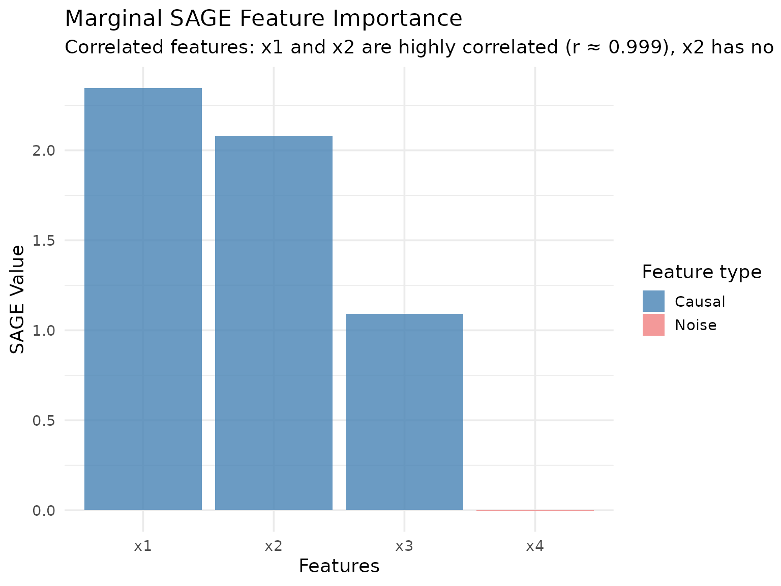
Marginal SAGE: Should show high importance for both x1 and x2 due to their correlation, even though x2 has no causal effect
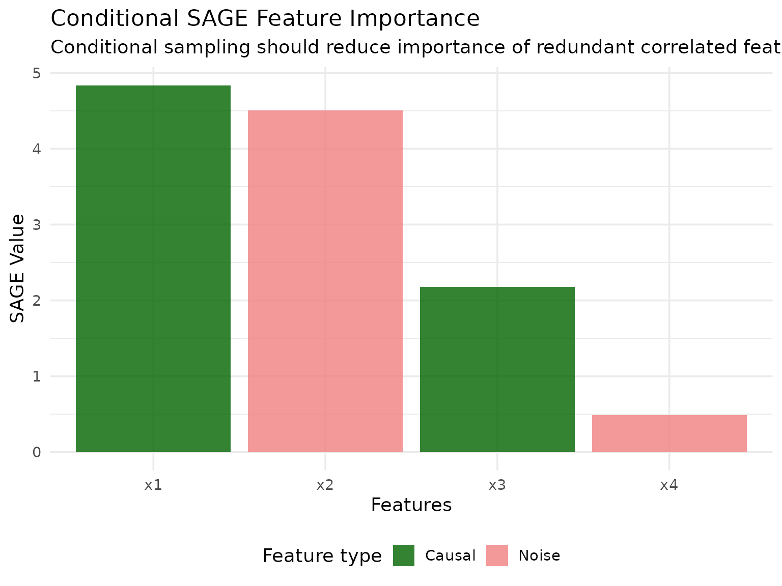
Conditional SAGE: Should show high importance for x1 but near-zero importance for x2 (correctly identifying the spurious predictor)

Let’s set up our learner and measure. We’ll use a random forest and instantiate a resampling to ensure both methods see the same data:

learner = lrn("regr.ranger", num.trees = 400)
measure = msr("regr.mse")
resampling = rsmp("holdout")
resampling$instantiate(task)

Marginal SAGE

Marginal SAGE marginalizes features independently by averaging predictions over a reference dataset. This is the standard SAGE implementation described in the original paper.

# Create Marginal SAGE instance
marginal_sage = MarginalSAGE$new(
  task = task,
  learner = learner,
  measure = measure,
  resampling = resampling,
  n_permutations = 30L,  # More permutations for stable results
  max_reference_size = 100L
)

# Compute SAGE values
marginal_sage$compute(batch_size = 5000L)
#> Evaluating 647 batches of size 5000
#> Evaluating ■                                  1% | ETA:  2m
#> 
#> Evaluating ■                                  2% | ETA:  2m
#> 
#> Evaluating ■■                                 4% | ETA:  2m
#> 
#> Evaluating ■■■                                6% | ETA:  2m
#> 
#> Evaluating ■■■■                               9% | ETA:  2m
#> 
#> Evaluating ■■■■                              12% | ETA:  2m
#> 
#> Evaluating ■■■■■                             14% | ETA:  2m
#> 
#> Evaluating ■■■■■■                            17% | ETA:  2m
#> 
#> Evaluating ■■■■■■■                           19% | ETA:  2m
#> 
#> Evaluating ■■■■■■■■                          22% | ETA:  2m
#> 
#> Evaluating ■■■■■■■■                          24% | ETA:  1m
#> 
#> Evaluating ■■■■■■■■■                         27% | ETA:  1m
#> 
#> Evaluating ■■■■■■■■■■                        29% | ETA:  1m
#> 
#> Evaluating ■■■■■■■■■■■                       32% | ETA:  1m
#> 
#> Evaluating ■■■■■■■■■■■                       34% | ETA:  1m
#> 
#> Evaluating ■■■■■■■■■■■■                      37% | ETA:  1m
#> 
#> Evaluating ■■■■■■■■■■■■■                     39% | ETA:  1m
#> 
#> Evaluating ■■■■■■■■■■■■■■                    42% | ETA:  1m
#> 
#> Evaluating ■■■■■■■■■■■■■■                    44% | ETA:  1m
#> 
#> Evaluating ■■■■■■■■■■■■■■■                   47% | ETA:  1m
#> 
#> Evaluating ■■■■■■■■■■■■■■■■                  49% | ETA:  1m
#> 
#> Evaluating ■■■■■■■■■■■■■■■■                  51% | ETA:  1m
#> 
#> Evaluating ■■■■■■■■■■■■■■■■■                 54% | ETA:  1m
#> 
#> Evaluating ■■■■■■■■■■■■■■■■■■                56% | ETA:  1m
#> 
#> Evaluating ■■■■■■■■■■■■■■■■■■■               59% | ETA:  1m
#> 
#> Evaluating ■■■■■■■■■■■■■■■■■■■               61% | ETA: 47s
#> 
#> Evaluating ■■■■■■■■■■■■■■■■■■■■              64% | ETA: 44s
#> 
#> Evaluating ■■■■■■■■■■■■■■■■■■■■■             66% | ETA: 41s
#> 
#> Evaluating ■■■■■■■■■■■■■■■■■■■■■■            69% | ETA: 37s
#> 
#> Evaluating ■■■■■■■■■■■■■■■■■■■■■■            71% | ETA: 34s
#> 
#> Evaluating ■■■■■■■■■■■■■■■■■■■■■■■           74% | ETA: 31s
#> 
#> Evaluating ■■■■■■■■■■■■■■■■■■■■■■■■          77% | ETA: 28s
#> 
#> Evaluating ■■■■■■■■■■■■■■■■■■■■■■■■■         79% | ETA: 25s
#> 
#> Evaluating ■■■■■■■■■■■■■■■■■■■■■■■■■         81% | ETA: 22s
#> 
#> Evaluating ■■■■■■■■■■■■■■■■■■■■■■■■■■        84% | ETA: 19s
#> 
#> Evaluating ■■■■■■■■■■■■■■■■■■■■■■■■■■■       87% | ETA: 16s
#> 
#> Evaluating ■■■■■■■■■■■■■■■■■■■■■■■■■■■■      89% | ETA: 13s
#> 
#> Evaluating ■■■■■■■■■■■■■■■■■■■■■■■■■■■■      91% | ETA: 10s
#> 
#> Evaluating ■■■■■■■■■■■■■■■■■■■■■■■■■■■■■     94% | ETA:  7s
#> 
#> Evaluating ■■■■■■■■■■■■■■■■■■■■■■■■■■■■■■    96% | ETA:  4s
#> 
#> Evaluating ■■■■■■■■■■■■■■■■■■■■■■■■■■■■■■■   99% | ETA:  1s
#> 
#> Evaluating ■■■■■■■■■■■■■■■■■■■■■■■■■■■■■■■  100% | ETA:  0s
#> Key: <feature>
#>    feature   importance
#>     <char>        <num>
#> 1:      x1  2.345195994
#> 2:      x2  2.081543369
#> 3:      x3  1.092772173
#> 4:      x4 -0.001768496

Let’s visualize the results:

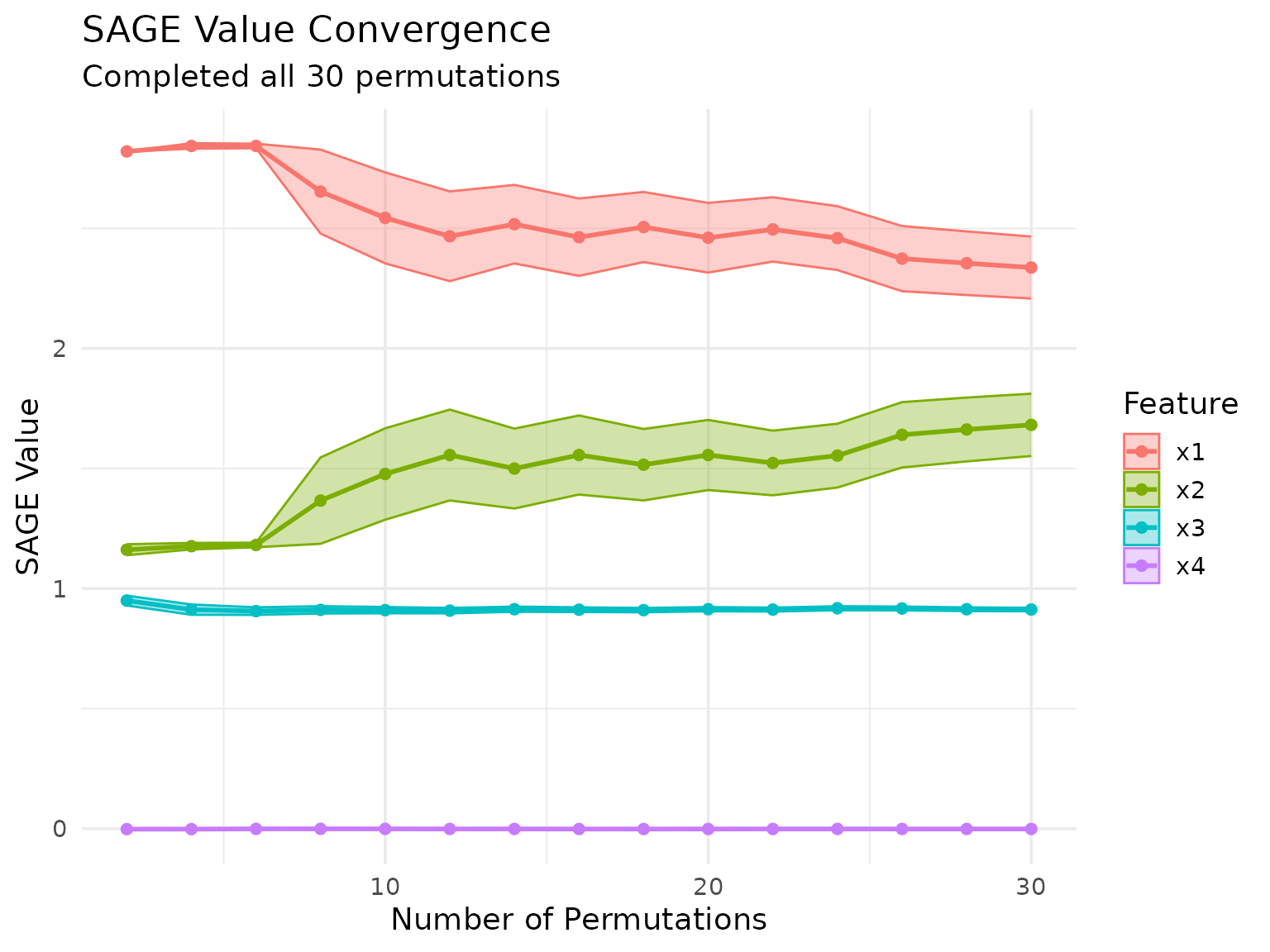
Conditional SAGE

Conditional SAGE uses conditional sampling (via ARF by default) to marginalize features while preserving dependencies between the remaining features. This can provide different insights, especially when features are correlated.

# Create Conditional SAGE instance
conditional_sage = ConditionalSAGE$new(
  task = task,
  learner = learner,
  measure = measure,
  resampling = resampling,
  n_permutations = 30L,
  max_reference_size = 100L
)
#> ℹ No <ConditionalSampler> provided, using <ARFSampler> with default settings.

# Compute SAGE values
conditional_sage$compute(batch_size = 5000L)
#> Evaluating 647 batches of size 5000
#> Evaluating ■                                  1% | ETA:  2m
#> Evaluating ■■                                 3% | ETA:  2m
#> Evaluating ■■■                                6% | ETA:  2m
#> Evaluating ■■■■                               9% | ETA:  2m
#> Evaluating ■■■■■                             12% | ETA:  2m
#> Evaluating ■■■■■                             15% | ETA:  1m
#> Evaluating ■■■■■■                            18% | ETA:  1m
#> Evaluating ■■■■■■■                           21% | ETA:  1m
#> Evaluating ■■■■■■■■                          24% | ETA:  1m
#> Evaluating ■■■■■■■■■                         26% | ETA:  1m
#> Evaluating ■■■■■■■■■■                        29% | ETA:  1m
#> Evaluating ■■■■■■■■■■■                       32% | ETA:  1m
#> Evaluating ■■■■■■■■■■■■                      35% | ETA:  1m
#> Evaluating ■■■■■■■■■■■■                      38% | ETA:  1m
#> Evaluating ■■■■■■■■■■■■■                     41% | ETA:  1m
#> Evaluating ■■■■■■■■■■■■■■                    44% | ETA:  1m
#> Evaluating ■■■■■■■■■■■■■■■                   47% | ETA:  1m
#> Evaluating ■■■■■■■■■■■■■■■■                  49% | ETA:  1m
#> Evaluating ■■■■■■■■■■■■■■■■■                 52% | ETA: 50s
#> Evaluating ■■■■■■■■■■■■■■■■■■                55% | ETA: 47s
#> Evaluating ■■■■■■■■■■■■■■■■■■                58% | ETA: 44s
#> Evaluating ■■■■■■■■■■■■■■■■■■■               61% | ETA: 41s
#> Evaluating ■■■■■■■■■■■■■■■■■■■■              64% | ETA: 38s
#> Evaluating ■■■■■■■■■■■■■■■■■■■■■             67% | ETA: 35s
#> Evaluating ■■■■■■■■■■■■■■■■■■■■■■            69% | ETA: 32s
#> Evaluating ■■■■■■■■■■■■■■■■■■■■■■■           72% | ETA: 29s
#> Evaluating ■■■■■■■■■■■■■■■■■■■■■■■■          75% | ETA: 26s
#> Evaluating ■■■■■■■■■■■■■■■■■■■■■■■■          78% | ETA: 23s
#> Evaluating ■■■■■■■■■■■■■■■■■■■■■■■■■         81% | ETA: 20s
#> Evaluating ■■■■■■■■■■■■■■■■■■■■■■■■■■        84% | ETA: 17s
#> Evaluating ■■■■■■■■■■■■■■■■■■■■■■■■■■■       87% | ETA: 14s
#> Evaluating ■■■■■■■■■■■■■■■■■■■■■■■■■■■■      89% | ETA: 11s
#> Evaluating ■■■■■■■■■■■■■■■■■■■■■■■■■■■■■     92% | ETA:  8s
#> Evaluating ■■■■■■■■■■■■■■■■■■■■■■■■■■■■■■    95% | ETA:  5s
#> Evaluating ■■■■■■■■■■■■■■■■■■■■■■■■■■■■■■    98% | ETA:  2s
#> Evaluating ■■■■■■■■■■■■■■■■■■■■■■■■■■■■■■■  100% | ETA:  0s
#> Key: <feature>
#>    feature importance
#>     <char>      <num>
#> 1:      x1  4.8350542
#> 2:      x2  4.5031386
#> 3:      x3  2.1808513
#> 4:      x4  0.4859302

Let’s visualize the conditional SAGE results:

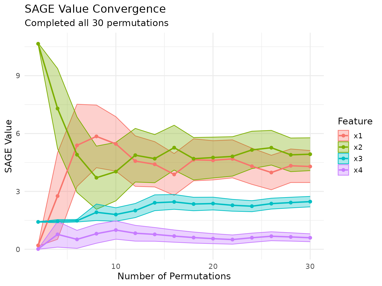
Comparison of Methods

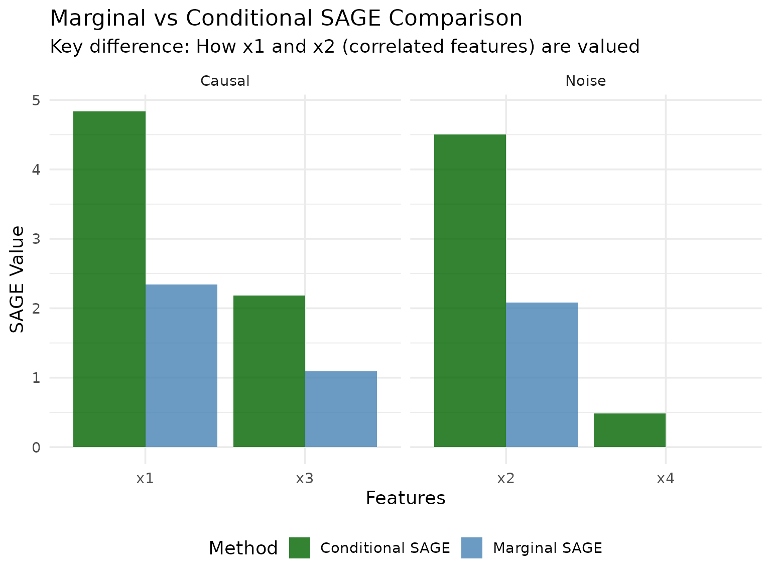
Let’s compare the two SAGE methods side by side:

Let’s also create a correlation plot to see how similar the rankings are:

#> `geom_smooth()` using formula = 'y ~ x'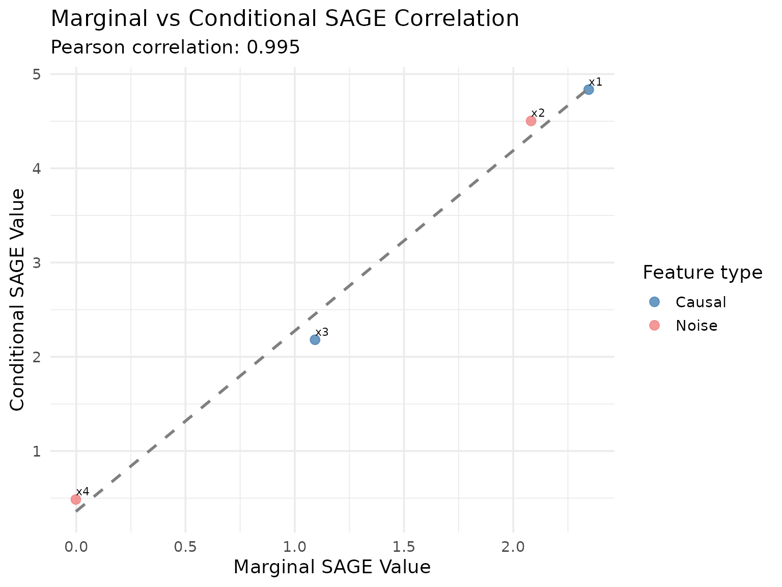

Interpretation

The results demonstrate the key difference between marginal and conditional SAGE:

Marginal SAGE treats each feature independently, so highly correlated features x1 and x2 both receive substantial importance scores reflecting their individual marginal contributions.
Conditional SAGE accounts for feature dependencies through conditional sampling. When marginalizing x1, it properly conditions on x2 (and vice versa), leading to lower importance scores for the correlated features since they provide redundant information.
Independent feature x3 shows similar importance in both methods since it doesn’t depend on other features.
Noise feature x4 correctly receives near-zero importance in both methods.

This pattern mirrors the difference between PFI and CFI: marginal methods show inflated importance for correlated features, while conditional methods provide a more accurate assessment of each feature’s unique contribution.

Comparison with PFI and CFI

For reference, let’s compare SAGE methods with the analogous PFI and CFI methods on the same data:

# Quick PFI and CFI comparison for context
pfi = PFI$new(task, learner, measure)
#> ℹ No <Resampling> provided, using holdout resampling with default ratio.
cfi = CFI$new(task, learner, measure) 
#> ℹ No <ConditionalSampler> provided, using <ARFSampler> with default settings.
#> ℹ No <Resampling> provided, using holdout resampling with default ratio.

pfi_results = pfi$compute()
cfi_results = cfi$compute()

# Create comparison data frame
method_comparison = data.frame(
  feature = rep(c("x1", "x2", "x3", "x4"), 4),
  importance = c(
    pfi_results$importance,
    cfi_results$importance,
    marginal_results$importance,
    conditional_results$importance
  ),
  method = rep(c("PFI", "CFI", "Marginal SAGE", "Conditional SAGE"), each = 4),
  approach = rep(c("Marginal", "Conditional", "Marginal", "Conditional"), each = 4)
)

# Create comparison plot
ggplot(method_comparison, aes(x = feature, y = importance, fill = method)) +
  geom_col(position = "dodge", alpha = 0.8) +
  scale_fill_manual(values = c(
    "PFI" = "lightblue", 
    "CFI" = "blue", 
    "Marginal SAGE" = "lightcoral", 
    "Conditional SAGE" = "darkred"
  )) +
  labs(
    title = "Comparison: PFI/CFI vs Marginal/Conditional SAGE",
    subtitle = "Both pairs show similar patterns: marginal methods inflate correlated feature importance",
    x = "Features", 
    y = "Importance Value",
    fill = "Method"
  ) +
  theme_minimal(base_size = 14) +
  theme(axis.text.x = element_text(angle = 45, hjust = 1))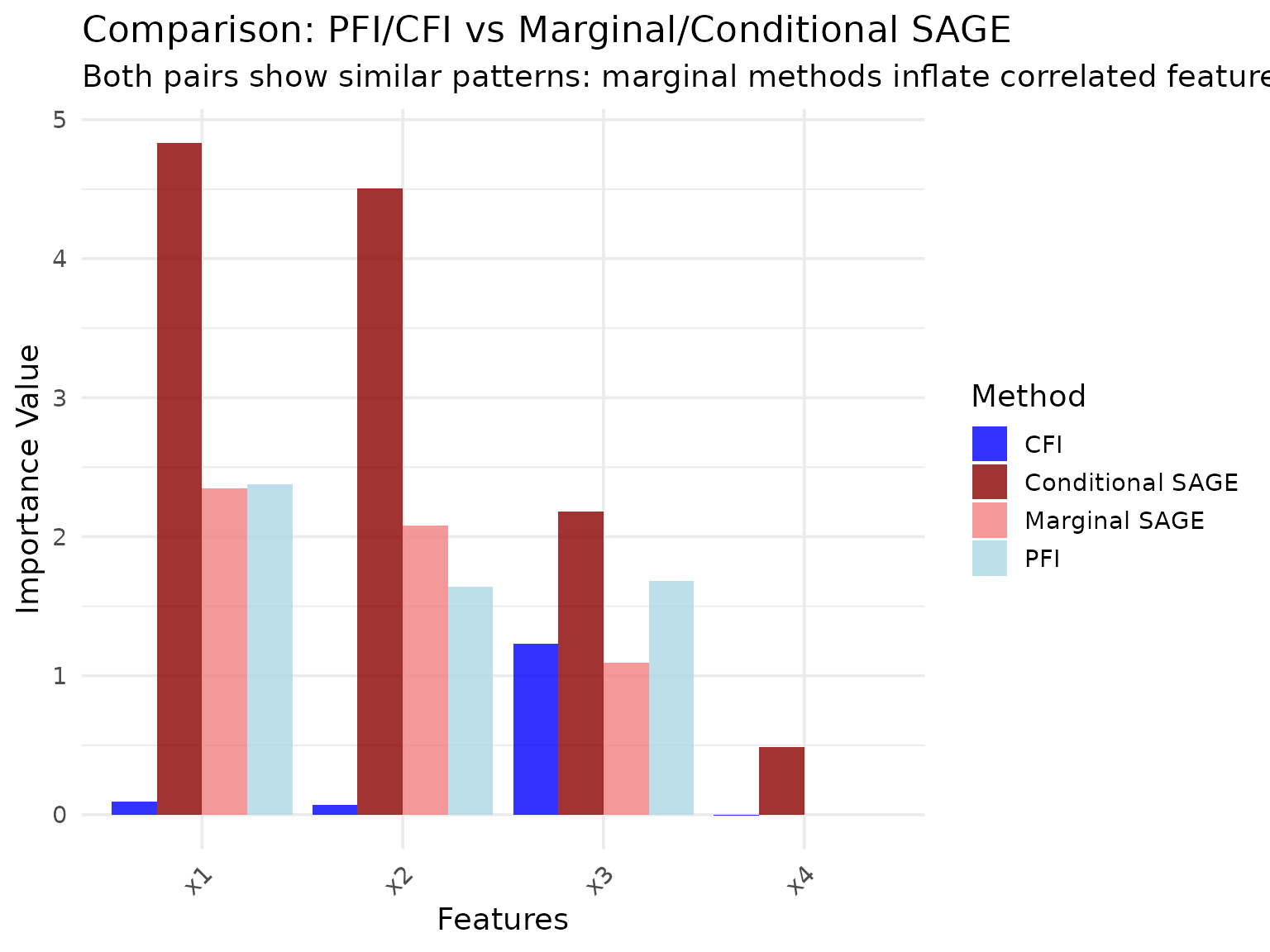

Key Observations:

Marginal methods (PFI, Marginal SAGE) both assign high importance to correlated features x1 and x2
Conditional methods (CFI, Conditional SAGE) both reduce importance for correlated features, accounting for redundancy
Independent feature x3 receives consistent importance across all methods
Noise feature x4 is correctly identified as unimportant by all methods

This demonstrates that the marginal vs conditional distinction is a fundamental concept that applies across different importance method families.