D.2 Beispiel nach Hilbe (2014 p. 211ff)

(Eigentlich kompliziertes Beispiel, weil 0 counts nicht möglich sind, müsste man truncated drangehen)

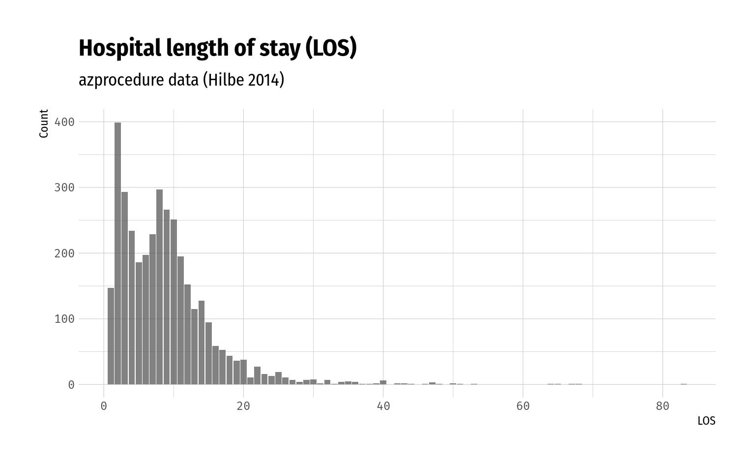
Grundlage ist der Datensatz azprocedure (siehe Abschnitt 1.1) zur Dauer des Krankenhausaufenthalts.

Zuerst werfen wir einen Blick auf die Daten und fitten ein reguläres Poissonmodell.

data(azprocedure, package = "COUNT")

describe_counts(azprocedure$los)

N	Missing	Mittelwert	Varianz	Range
3589	0	8.83	47.97	[1, 83]

# Barchart: So grob poissonverteilt?
ggplot(data = azprocedure, aes(x = los)) +
  geom_bar(alpha = .75) +
  labs(
    title = "Hospital length of stay (LOS)",
    subtitle = "azprocedure data (Hilbe 2014)",
    x = "LOS", y = "Count" 
  )

# Model fit
model_azproc <- glm(los ~ procedure + sex + admit, 
                    data = azprocedure, family = poisson())
 
# Model output (ohne exponentierte Koeffizienten)
pander(model_azproc)

Fitting generalized (poisson/log) linear model: los ~ procedure + sex + admit
	Estimate	Std. Error	z value	Pr(>\|z\|)
(Intercept)	1.491	0.01539	96.91	0
procedure	0.9574	0.01218	78.61	0
sex	-0.1302	0.01179	-11.04	2.408e-28
admit	0.3331	0.0121	27.52	1.11e-166

# Pearson Dispersion:
dispersion(model_azproc)

#> X-squared(3585) = 11588.08
#> Pearson Dispersion = 3.232

Der Dispersionsindex lässt auf overdispersion schließen.
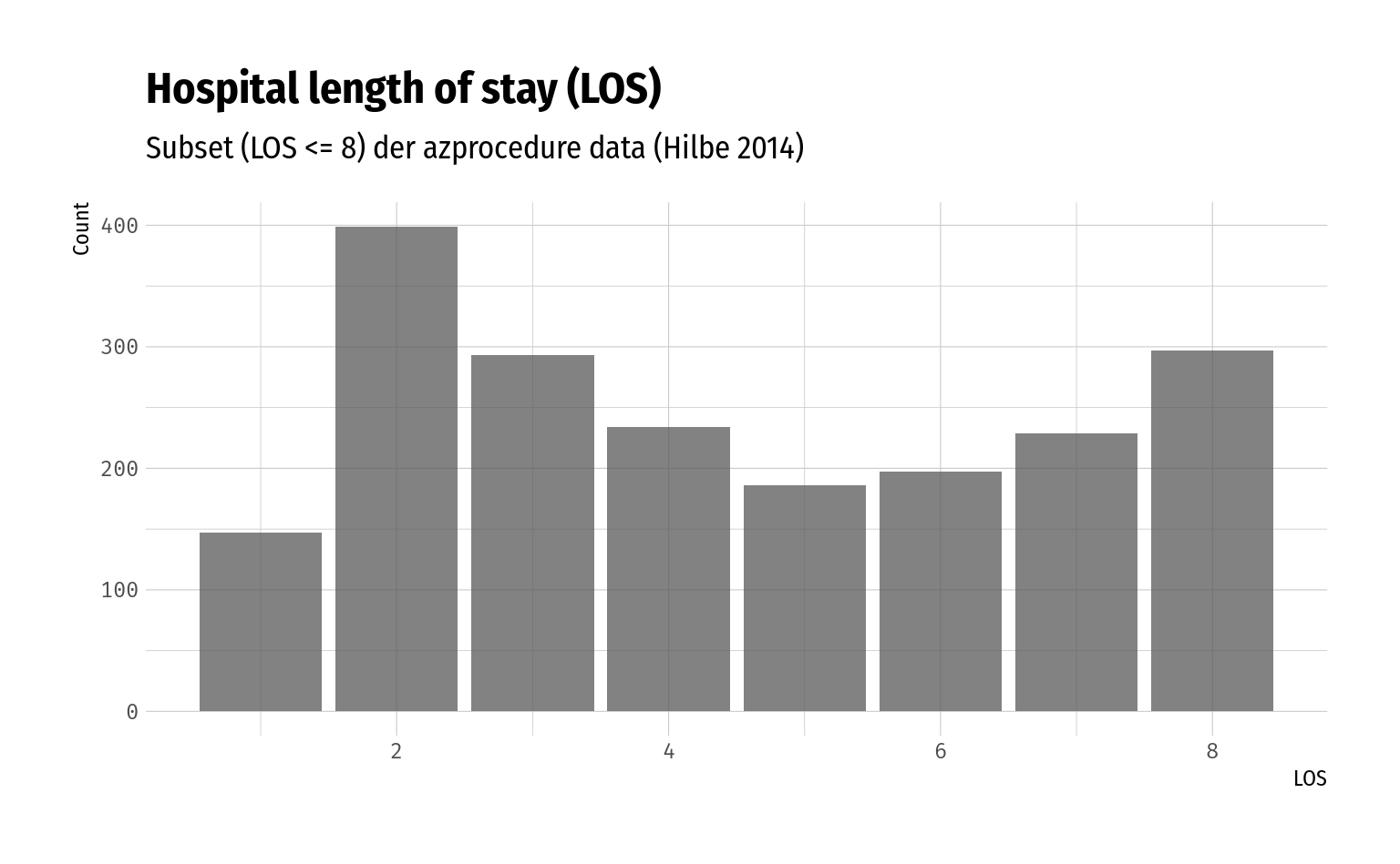
Betrachten wir ein Subset der Daten, indem wir nur Beobachtungen mit \(\mathtt{LOS} \le 8\) betrachten, erhalten wir ein anderes Bild:

azprocedure_subset <- subset(azprocedure, los <= 8)

describe_counts(azprocedure_subset$los)

N	Missing	Mittelwert	Varianz	Range
1982	0	4.47	5.34	[1, 8]

# Barchart
ggplot(data = azprocedure_subset, aes(x = los)) +
  geom_bar(alpha = .75) +
  labs(
    title = "Hospital length of stay (LOS)",
    subtitle = "Subset (LOS <= 8) der azprocedure data (Hilbe 2014)",
    x = "LOS", y = "Count" 
  )

model_azproc_u <- glm(los ~ procedure + sex + admit, 
                      data = azprocedure_subset, family = poisson())

pander(model_azproc_u)

Fitting generalized (poisson/log) linear model: los ~ procedure + sex + admit
	Estimate	Std. Error	z value	Pr(>\|z\|)
(Intercept)	1.187	0.02498	47.52	0
procedure	0.731	0.02398	30.48	4.848e-204
sex	-0.06892	0.02294	-3.004	0.00266
admit	0.3097	0.02236	13.85	1.286e-43

dispersion(model_azproc_u)

#> X-squared(1978) = 1562.75
#> Pearson Dispersion = 0.790

In diesem Fall haben wir es mit underdispersion zu tun, also versuchen wir es mal mit der GP:

library(VGAM)
library(gamlss)

mod_gp_vgam <- vglm(los ~ procedure + sex + admit, data = azprocedure_subset, family = genpoisson())

mod_gp_gamlss <- gamlss(los ~ procedure + sex + admit, data = azprocedure_subset, family = GPO())

#> GAMLSS-RS iteration 1: Global Deviance = 7969.342 
#> GAMLSS-RS iteration 2: Global Deviance = 7961.567 
#> GAMLSS-RS iteration 3: Global Deviance = 7961.567

summary(mod_gp_vgam)

#> 
#> Call:
#> vglm(formula = los ~ procedure + sex + admit, family = genpoisson(), 
#>     data = azprocedure_subset)
#> 
#> Pearson residuals:
#>                        Min      1Q   Median     3Q   Max
#> rhobitlink(lambda) -0.6573 -0.5912 -0.28788 0.2773 6.782
#> loglink(theta)     -2.3158 -0.6304  0.07304 0.8734 1.627
#> 
#> Coefficients: 
#>               Estimate Std. Error z value Pr(>|z|)    
#> (Intercept):1 -0.24021    0.03523  -6.819 9.16e-12 ***
#> (Intercept):2  1.30125    0.02766  47.042  < 2e-16 ***
#> procedure      0.71846    0.02143  33.521  < 2e-16 ***
#> sex           -0.06760    0.02043  -3.308 0.000939 ***
#> admit          0.31193    0.01993  15.652  < 2e-16 ***
#> ---
#> Signif. codes:  0 '***' 0.001 '**' 0.01 '*' 0.05 '.' 0.1 ' ' 1
#> 
#> Names of linear predictors: rhobitlink(lambda), loglink(theta)
#> 
#> Log-likelihood: -3956.379 on 3959 degrees of freedom
#> 
#> Number of Fisher scoring iterations: 6 
#> 
#> No Hauck-Donner effect found in any of the estimates

summary(mod_gp_gamlss)

#> ******************************************************************
#> Family:  c("GPO", "Generalised Poisson") 
#> 
#> Call:  gamlss(formula = los ~ procedure + sex + admit, family = GPO(),  
#>     data = azprocedure_subset) 
#> 
#> Fitting method: RS() 
#> 
#> ------------------------------------------------------------------
#> Mu link function:  log
#> Mu Coefficients:
#>             Estimate Std. Error t value Pr(>|t|)    
#> (Intercept)  1.18687    0.02980  39.824   <2e-16 ***
#> procedure    0.73075    0.03959  18.456   <2e-16 ***
#> sex         -0.06892    0.02643  -2.607   0.0092 ** 
#> admit        0.30974    0.02750  11.264   <2e-16 ***
#> ---
#> Signif. codes:  0 '***' 0.001 '**' 0.01 '*' 0.05 '.' 0.1 ' ' 1
#> 
#> ------------------------------------------------------------------
#> Sigma link function:  log
#> Sigma Coefficients:
#>             Estimate Std. Error t value Pr(>|t|)
#> (Intercept)   -36.04    2246.20  -0.016    0.987
#> 
#> ------------------------------------------------------------------
#> No. of observations in the fit:  1982 
#> Degrees of Freedom for the fit:  5
#>       Residual Deg. of Freedom:  1977 
#>                       at cycle:  3 
#>  
#> Global Deviance:     7961.567 
#>             AIC:     7971.567 
#>             SBC:     7999.527 
#> ******************************************************************

Beispiel aus Hilbe 2014. Eigentlich sollte \(\delta \approx -0.1195\) und \(\theta = \frac{1}{(1 - \delta)^2} \approx 0.799\)