library(xplainfi)
library(mlr3learners)
#> Loading required package: mlr3

# Data manip and visualization
library(data.table)
library(ggplot2)
There are multiple (work in progress) inference possible with the underlying implementation, but the API around them is still being worked out.
Setup
We use a simple linear DGP for demonstration purposes where
- \(X_1\) and \(X_2\) are strongly correlated (r = 0.7)
- \(X_1\) and \(X_3\) has an effect on Y
- \(X_2\) and \(X_4\) don’t have an effect
task = sim_dgp_correlated(n = 2000, r = 0.7)
learner = lrn("regr.ranger", num.trees = 500)
measure = msr("regr.mse")
DAG for correlated features DGP
Variance-correction
When we calculate PFI using an appropriate resampling, such as subsampling with 15 repeats, we can use the approach recommended by Molnar et al. (2023) based on the proposed correction by Nadeay & Bengio (2003).
By default, any importance measures’ $importance()
method will not output any variances or confidence intervals, it will
merely compute averages over resampling iterations and repeats within
resamplings (iter_perm here).
pfi = PFI$new(
    task = task,
    learner = learner,
    resampling = rsmp("subsampling", repeats = 15),
    measure = measure,
    iters_perm = 10 # for stability within resampling iters
)

pfi$compute()
pfi$importance()
#> Key: <feature>
#>    feature   importance
#>     <char>        <num>
#> 1:      x1  6.444709393
#> 2:      x2  0.097777103
#> 3:      x3  1.801488945
#> 4:      x4 -0.001099328
If we want unadjusted confidence intervals we can ask for them, but note these are too narrow / optimistic and hence invalid for inference:
pfi_ci_raw = pfi$importance(ci_method = "raw")
pfi_ci_raw
#> Key: <feature>
#>    feature   importance           se   conf_lower   conf_upper
#>     <char>        <num>        <num>        <num>        <num>
#> 1:      x1  6.444709393 0.0710846455  6.292247992  6.597170794
#> 2:      x2  0.097777103 0.0040374343  0.089117668  0.106436538
#> 3:      x3  1.801488945 0.0163236399  1.766478220  1.836499671
#> 4:      x4 -0.001099328 0.0003169572 -0.001779133 -0.000419522
Analogously we can retrieve the Nadeau & Bengio-adjusted standard errors and derived confidence intervals which were demonstrated to have better (but still imperfect) coverage:
pfi_ci_corrected = pfi$importance(ci_method = "nadeau_bengio")
pfi_ci_corrected
#> Key: <feature>
#>    feature   importance           se  conf_lower   conf_upper
#>     <char>        <num>        <num>       <num>        <num>
#> 1:      x1  6.444709393 0.2073141539  6.00006476 6.8893540305
#> 2:      x2  0.097777103 0.0117749378  0.07252237 0.1230318328
#> 3:      x3  1.801488945 0.0476069279  1.69938224 1.9035956504
#> 4:      x4 -0.001099328 0.0009243869 -0.00308194 0.0008832851
Non-parametric alternative: Empirical quantiles
Both "raw" and "nadeau_bengio" methods
assume normally distributed importance scores and use parametric
confidence intervals based on the t-distribution. As a non-parametric
alternative, we can use empirical quantiles that directly use the
resampling distribution to construct confidence-like intervals.
Like the Nadeau & Bengio approach, this method requires independent resampling splits. This means it works with subsampling or bootstrap, but not with cross-validation.
pfi_ci_quantile = pfi$importance(ci_method = "quantile")
pfi_ci_quantile
#> Key: <feature>
#>    feature   importance   conf_lower   conf_upper
#>     <char>        <num>        <num>        <num>
#> 1:      x1  6.444709393  5.981573776 6.8770935941
#> 2:      x2  0.097777103  0.075868045 0.1226624975
#> 3:      x3  1.801488945  1.692275614 1.8953539522
#> 4:      x4 -0.001099328 -0.003684845 0.0005401245
To highlight the differences between parametric and non-parametric approaches, we visualize all methods:
pfi_cis = rbindlist(
    list(
        pfi_ci_raw[, type := "raw"],
        pfi_ci_corrected[, type := "nadeau_bengio"],
        pfi_ci_quantile[, type := "quantile"]
    ),
    fill = TRUE
)

ggplot(pfi_cis, aes(y = feature, color = type)) +
    geom_errorbar(
        aes(xmin = conf_lower, xmax = conf_upper),
        position = position_dodge(width = 0.6),
        width = .5
    ) +
    geom_point(aes(x = importance), position = position_dodge(width = 0.6)) +
    scale_color_brewer(palette = "Set2") +
    labs(
        title = "Parametric & non-parametric CI methods",
        subtitle = "RF with 15 subsampling iterations",
        color = NULL
    ) +
    theme_minimal(base_size = 14) +
    theme(legend.position = "bottom")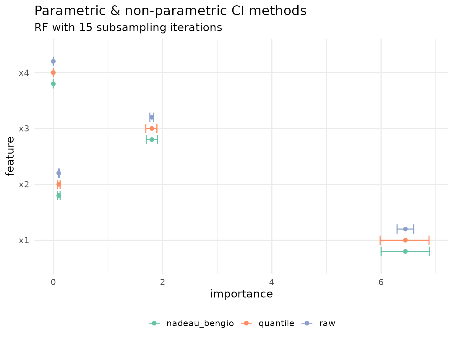
The results highlight just how optimistic the unadjusted, raw confidence intervals are.
Conditional predictive impact (CPI)
CPI is implemented by the cpi
package, and provides conditional variable importance using
knockoffs. It works with mlr3 and its output on our data
looks like this:
cpi_res = cpi(
    task = task,
    learner = learner,
    resampling = resampling,
    measure = measure,
    test = "t"
)
setDT(cpi_res)
setnames(cpi_res, "Variable", "feature")
cpi_res[, method := "CPI"]

cpi_res
#>    feature           CPI           SE   test statistic      estimate
#>     <char>         <num>        <num> <char>     <num>         <num>
#> 1:      x1  4.4905247594 0.1393416714      t 32.226718  4.4905247594
#> 2:      x2 -0.0026748965 0.0023132871      t -1.156318 -0.0026748965
#> 3:      x3  1.7350915247 0.0551007024      t 31.489463  1.7350915247
#> 4:      x4 -0.0009994758 0.0009142715      t -1.093194 -0.0009994758
#>          p.value        ci.lo method
#>            <num>        <num> <char>
#> 1: 3.644769e-184  4.261221841    CPI
#> 2:  8.761554e-01 -0.006481679    CPI
#> 3: 2.156035e-177  1.644416914    CPI
#> 4:  8.627797e-01 -0.002504016    CPI
CPI with knockoffs
Since xplainfi also includes knockoffs via the
KnockoffSampler and the
KnockoffGaussianSampler, the latter implementing the second
order Gaussian knockoffs also used by default in cpi, we
can recreate its results using CFI with the corresponding
sampler.
CFI with a knockoff sampler supports CPI inference
directly via ci_method = "cpi":
knockoff_gaussian = KnockoffGaussianSampler$new(task)

cfi = CFI$new(
    task = task,
    learner = learner,
    resampling = resampling,
    measure = measure,
    sampler = knockoff_gaussian
)

cfi$compute()

# CPI uses observation-wise losses with one-sided t-test
cfi_cpi_res = cfi$importance(ci_method = "cpi")
cfi_cpi_res
#> Key: <feature>
#>    feature    importance           se   statistic       p.value   conf_lower
#>     <char>         <num>        <num>       <num>         <num>        <num>
#> 1:      x1  4.6485211373 0.1412096720 32.91928289 1.430822e-190  4.416144207
#> 2:      x2 -0.0002372201 0.0029839960 -0.07949746  5.316775e-01 -0.005147732
#> 3:      x3  1.8639780917 0.0561726066 33.18304428 5.072022e-193  1.771539538
#> 4:      x4 -0.0002621368 0.0007881572 -0.33259452  6.302624e-01 -0.001559141
#>    conf_upper
#>         <num>
#> 1:        Inf
#> 2:        Inf
#> 3:        Inf
#> 4:        Inf

# Rename columns to match cpi package output for comparison
setnames(cfi_cpi_res, c("importance", "conf_lower"), c("CPI", "ci.lo"))
cfi_cpi_res[, method := "CFI+Knockoffs"]
The results should be very similar to those computed by
cpi(), so let’s compare them:
rbindlist(list(cpi_res, cfi_cpi_res), fill = TRUE) |>
    ggplot(aes(y = feature, x = CPI, color = method)) +
    geom_point(position = position_dodge(width = 0.3)) +
    geom_errorbar(
        aes(xmin = CPI, xmax = ci.lo),
        position = position_dodge(width = 0.3),
        width = 0.5
    ) +
    scale_color_brewer(palette = "Dark2") +
    labs(
        title = "CPI and CFI with Knockoff sampler",
        subtitle = "RF with 5-fold CV",
        color = NULL
    ) +
    theme_minimal(base_size = 14) +
    theme(legend.position = "top")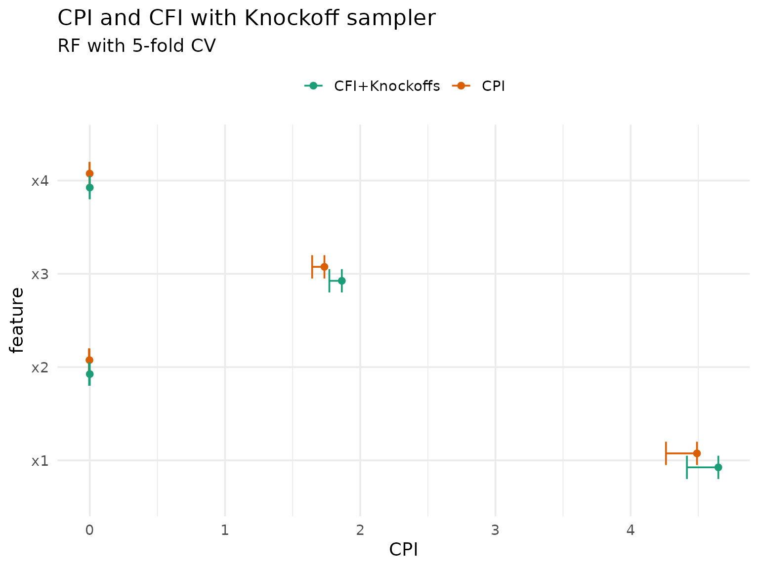
A noteable caveat of the knockoff approach is that they are not readily available for mixed data (with categorical features).
CPI with ARF
An alternative is available using ARF as conditional sampler rather than knockoffs (CITE cARFi), which we can perform analogously:
arf_sampler = ARFSampler$new(
    task = task,
    finite_bounds = "local",
    min_node_size = 20,
    epsilon = 1e-15
)

cfi_arf = CFI$new(
    task = task,
    learner = learner,
    resampling = resampling,
    measure = measure,
    sampler = arf_sampler
)

cfi_arf$compute()

# CPI uses observation-wise losses with one-sided t-test
cfi_arf_res = cfi_arf$importance(ci_method = "cpi")
cfi_arf_res
#> Key: <feature>
#>    feature   importance           se statistic       p.value    conf_lower
#>     <char>        <num>        <num>     <num>         <num>         <num>
#> 1:      x1  4.149913006 0.1377986710 30.115769 6.416347e-165  3.9231492740
#> 2:      x2  0.005623742 0.0036623984  1.535535  6.240533e-02 -0.0004031606
#> 3:      x3  1.703418858 0.0547593855 31.107341 6.653459e-174  1.6133059238
#> 4:      x4 -0.002416235 0.0007663808 -3.152786  9.991794e-01 -0.0036774039
#>    conf_upper
#>         <num>
#> 1:        Inf
#> 2:        Inf
#> 3:        Inf
#> 4:        Inf

# Rename columns to match cpi package output for comparison
setnames(cfi_arf_res, c("importance", "conf_lower"), c("CPI", "ci.lo"))
cfi_arf_res[, method := "CFI+ARF"]
We can now compare all three methods:
rbindlist(list(cpi_res, cfi_cpi_res, cfi_arf_res), fill = TRUE) |>
    ggplot(aes(y = feature, x = CPI, color = method)) +
    geom_point(position = position_dodge(width = 0.3)) +
    geom_errorbar(
        aes(xmin = CPI, xmax = ci.lo),
        position = position_dodge(width = 0.3),
        width = 0.5
    ) +
    scale_color_brewer(palette = "Dark2") +
    labs(
        title = "CPI and CFI with Knockoffs and ARF",
        subtitle = "RF with 5-fold CV",
        color = NULL
    ) +
    theme_minimal(base_size = 14) +
    theme(legend.position = "top")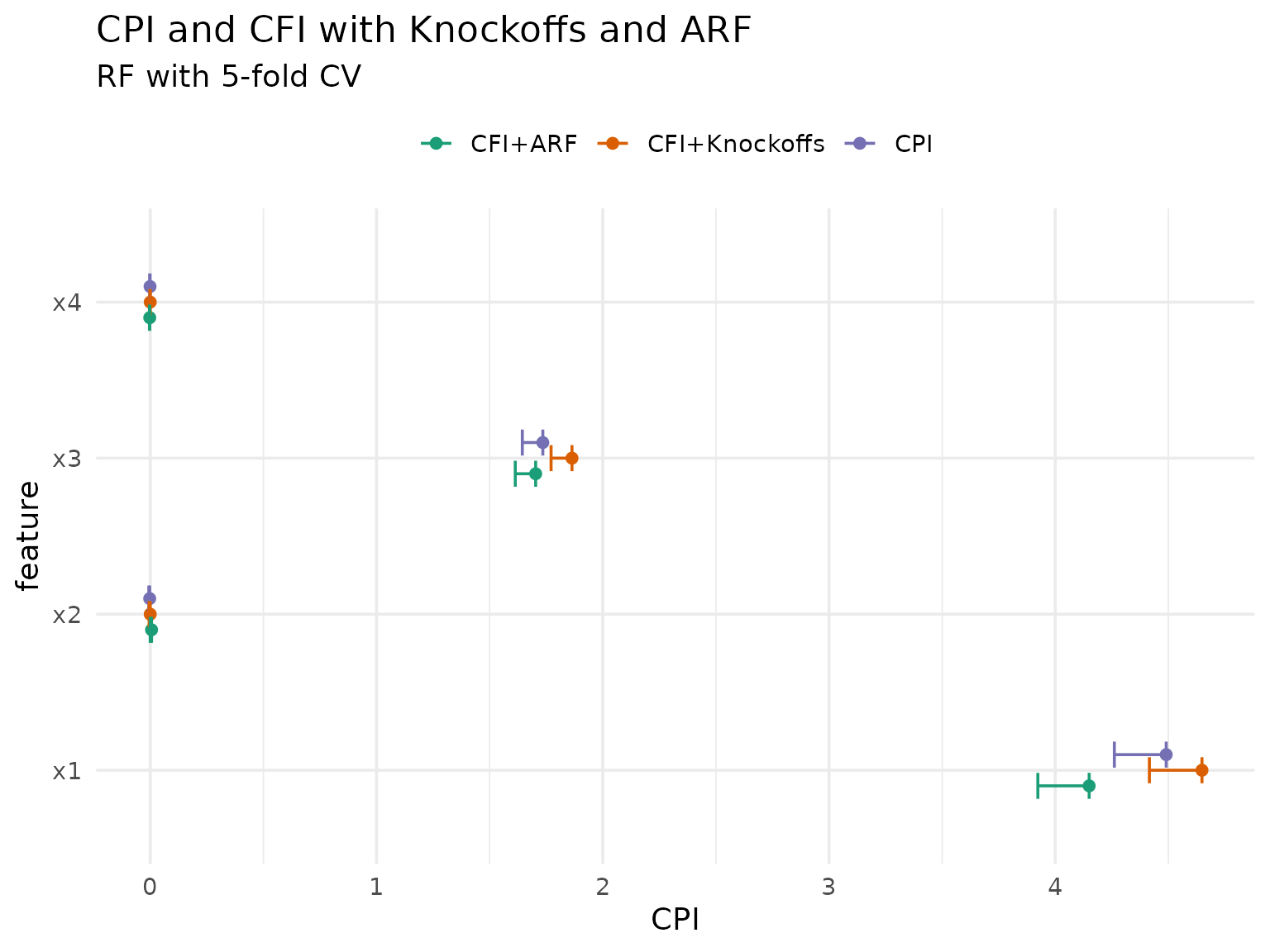
As expected, the ARF-based approach differs more from both knockoff-based approaches, but they are all roughly in agreement.
Note: xplainfi will gain a dedicated
interface to perform CPI, but the API is yet to be worked out.
LOCO (WIP)
(CITATION) proposed inference for LOCO using the median absolute differences of the baseline- and post-refit loss differences
\[ \theta_j = \mathrm{med}\left( |Y - \hat{f}_{n_1}^{-j}(X)| - |Y - \hat{f}_{n_1}(X)| \big| D_1 \right) \]
If we apply LOCO as implemented in xplainfi
using the median absolute error (MAE) as our measure including the
median as the aggregation function, we unfortunately get something else,
though:
measure_mae = msr("regr.mae")
measure_mae$aggregator = median

loco = LOCO$new(
    task = task,
    learner = learner,
    resampling = rsmp("cv", folds = 3),
    measure = measure_mae
)

loco$compute()
loco$importance()
#> Key: <feature>
#>    feature importance
#>     <char>      <num>
#> 1:      x1 0.99962897
#> 2:      x2 0.04442239
#> 3:      x3 0.63009668
#> 4:      x4 0.04054127
This is not exactly what the authors propose,
because $score() calculates the aggregation function
(median) for each resampling iteration first, and takes the
difference afterwards, i.e.
\[ \theta_j = \mathrm{med}\left(|Y - \hat{f}_{n_1}^{-j}(X)|\right) - \mathrm{med}\left(|Y - \hat{f}_{n_1}(X)| \big| D_1 \right) \]
In the default case where the arithemtic mean is used, it does not matter whether we calculate the difference of the means or the mean of the differences, but using the median it does.
We can, however, reconstruct it by using the observation-wise losses (in this case, the absolute error):
loco_obsloss = loco$obs_loss()
head(loco_obsloss)
#>    feature iter_rsmp iter_refit row_ids loss_baseline loss_post obs_importance
#>     <char>     <int>      <num>   <int>         <num>     <num>          <num>
#> 1:      x1         1          1       5    0.26081483 1.0828744      0.8220595
#> 2:      x1         1          1       8    0.07863945 1.4662680      1.3876286
#> 3:      x1         1          1      18    0.12976167 0.9243277      0.7945660
#> 4:      x1         1          1      19    0.14154518 1.3045495      1.1630043
#> 5:      x1         1          1      20    0.25832021 0.4959166      0.2375964
#> 6:      x1         1          1      21    0.18253098 0.7409787      0.5584477
obs_importance here refers to the difference
loss_post - loss_baseline, so
-
loss_baseline$ = |Y - _{n_1}(X)|$ -
loss_post$ = |Y - _{n_1}^{-j}(X)|$ obs_importance = loss_post - loss_baseline
Which means by taking the median for each feature \(j\) within each resampling iteration, we can construct \(\theta_j(D_1)\) as proposed, for each set \(D_k\) where \(k\) is the resampling iteration:
loco_thetas = loco_obsloss[, list(theta = median(obs_importance)), by = c("feature", "iter_rsmp")]
loco_thetas
#>     feature iter_rsmp      theta
#>      <char>     <int>      <num>
#>  1:      x1         1 0.89502517
#>  2:      x1         2 0.86756440
#>  3:      x1         3 0.77528481
#>  4:      x2         1 0.02726682
#>  5:      x2         2 0.02843028
#>  6:      x2         3 0.01773224
#>  7:      x3         1 0.51379135
#>  8:      x3         2 0.54167072
#>  9:      x3         3 0.56786544
#> 10:      x4         1 0.01789627
#> 11:      x4         2 0.03044097
#> 12:      x4         3 0.02302404
The authors then propose to construct distribution-free confidence intervals, e.g. using a sign- or Wilcoxon test We can for example use [wilcoxon.test] to compute confidence intervals around the estimated pseudo-median:
loco_wilcox_ci = loco_obsloss[,
    {
        tt <- wilcox.test(
            obs_importance,
            conf.int = TRUE,
            conf.level = 0.95
        )
        .(
            statistic = tt$statistic,
            estimate = tt$estimate, # the pseudomedian importance
            p.value = tt$p.value,
            conf_lower = tt$conf.int[1],
            conf_upper = tt$conf.int[2]
        )
    },
    by = feature
]

loco_wilcox_ci
#>    feature statistic   estimate       p.value conf_lower conf_upper
#>     <char>     <num>      <num>         <num>      <num>      <num>
#> 1:      x1   1943253 0.92960910 1.151861e-291 0.88933069 0.97052252
#> 2:      x2   1262272 0.03119993  3.880922e-24 0.02514172 0.03730949
#> 3:      x3   1891407 0.59426242 1.067356e-260 0.56662125 0.62207703
#> 4: x4 1351954 0.03074982 3.657070e-42 0.02623189 0.03538269Note: The above approach needs checking with the literature to ensure it’s actually corresponding to what was proposed and the results are valid.
The main point of this section is to illustrate that the availability of the intermediate parts (i.e. obs losses) and flexibility regarding the used measure allows for flexibility in terms of inference.